Levered ETFs for the Long Run?

By Corey Hoffstein, Newfound Research

Early last month, we published a piece titled Portable Beta: Making the Most of the Returns You’re Already Getting, in which we outlined an argument whereby investors should focus on capital efficiency. We laid out four ways in which we believe that investors can achieve greater efficiency:

Reduce fees to take home more of what you earn.
Express active views more purely so that we are not caught paying active management prices for closet beta.
Focus on risk management by “diversifying your diversifiers” with strategies like trend following that can help increase exposure to higher return asset classes without necessarily increasing the overall portfolio risk profile.
Utilize modest leverage so that investors can create more risk-efficient portfolios without necessarily sacrificing potential return.

Unfortunately, for many investors, access to true leverage – either through borrowing or the use of derivatives – may be beyond their means. Fortunately, there are a number of ETFs available today that allow investors to access leverage in a packaged manner.

Wait, Aren’t Levered ETFs Dangerous?

Levered ETFs have quite a reputation, and not a good one at that. A quick search will result in numerous articles that tell you why they are a dangerous, bad idea. They are pejoratively dismissed as “trading vehicles,” unsuitable for “buy and hold.”

Most often, the negative publicity hinges on the concept of volatility decay (or, sometimes “volatility drag”). To illuminate this concept, let’s assume there is a stock that can only go up either +X% or down –X%. Thus, in any two-day period, we have the following growth in our wealth:

	Up	Down
Up	(1 + X%)(1 + X%)	(1 – X%)(1 + X%)
Down	(1 + X%)(1 – X%)	(1 – X%)(1 – X%)

If we expand out the returns, we are left with:

	Up	Down
Up	1 + 2X% + X%²	1 – X%²
Down	1 – X%²	1 – 2X% + X%²

Note that in the case where the stock went up +X% and then down -X% (or down –X% and then up +X%), we did not end up back at our starting wealth. Rather, we ended up with a loss of -X%².

On the other hand, we can see that when the stock goes the same direction, we actually outperform twice the daily return by +X%².

What’s going on here?

It is nothing more than the math of compound returns. The returns of the second day compound the returns of the first.

The effect earns the moniker volatility decay because in return environments that are mean-reversionary (e.g. positive returns follow negative returns, and vice versa), our capital decays due to the -X%² term.

Note, however, that we haven’t even introduced leverage into the scenario yet. This drag is not unique to levered ETFs: it is just the math of compounding returns. Why it gets brought up so frequently with respect to levered ETFs is because the leverage can accentuate it. Consider what happens if we introduce a daily leverage factor of L:

	Up	Down
Up	1 + 2LX% + L²X%²	1 – L²X%²
Down	1 – L²X%²	1 – 2LX% + L²X%²

When L=1, we have a standard long-only investment. When L=2, we have our 2X daily levered ETFs. What we see is that when L=1, our drag is simply –X%². When L=2, however, our drag is 4X%². When L=3, the drag skyrockets to 9X%². Of course, the so-called drag turns into a benefit in trending markets (whether positive or negative).

So why do we not see this same effect when we use traditional leverage? After all, are these ETFs not using leverage under the hood to achieve their returns?

The answer lies in the daily reset. Note that these ETFs aim to give you a multiple of returns every day. The same is not true if we simply lever our notional exposure and never reset it. By “reset,” we mean pay back what we owe and re-borrow capital in order to maintain our leverage ratio.

To achieve 2X daily returns, the levered ETFs basically borrow their NAV, invest in the asset class, and then pay back what they borrowed. Hence, every day they reset how much they borrow.

If we never reset, however, the proportion of our capital that is levered varies over time. Consider, for example, investing $10,000 of our own capital in the SPDR S&P 500 ETF and borrowing another $10,000 to invest alongside (for convenience, we’re going to assume zero borrowing cost). As the market has gone up over time, the initial $10,000 borrowed becomes a smaller and smaller proportion of our capital.

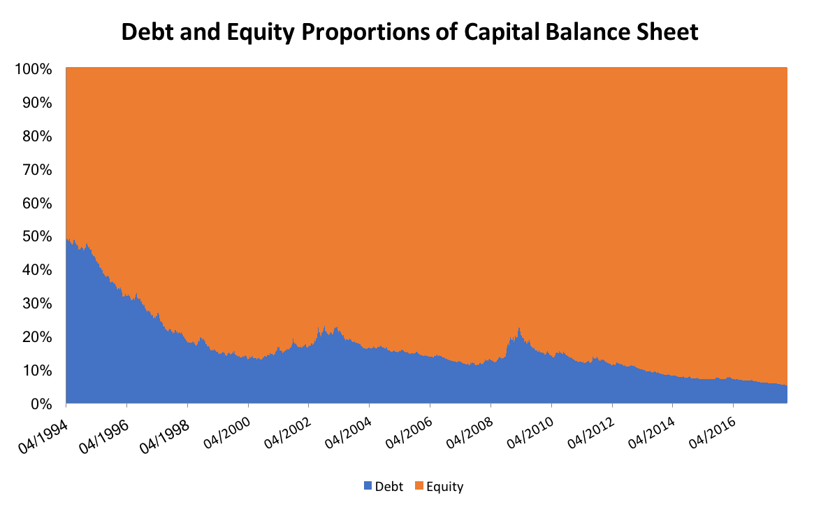
Source: CSI. Calculations by Newfound Research. Assumes portfolio applies 100% notional leverage applied to SPDR S&P 500 ETF (“SPY”) at inception of ETF. Assumes zero cost of leverage.

This happens because while we owe the initial $10,000 back, the returns made on that $10,000 are ours to keep. In the beginning, our portfolio will behave very much like a 2X daily levered ETF. As the market trends upward over time, however, we not only compound our own capital, but compound our gains on the levered capital. This causes our actual leverage to decline over time. As a result, our daily returns will gradually converge towards that of the market.

In practice, of course, there would be a cost associated with borrowing the $10,000. However, the same fact pattern applies so long as the growth of the portfolio exceeds the cost of leverage.

Resetting, therefore, is a necessary component of maintaining leverage. On the one hand, we have daily resets, which keeps our leverage proportion constant. On the other hand, we have “never reset,” which will decay the leverage proportion over time (assuming the portfolio grows faster than the cost of leverage). There are, of course, shades of gray as well. Consider a 1-year reset:

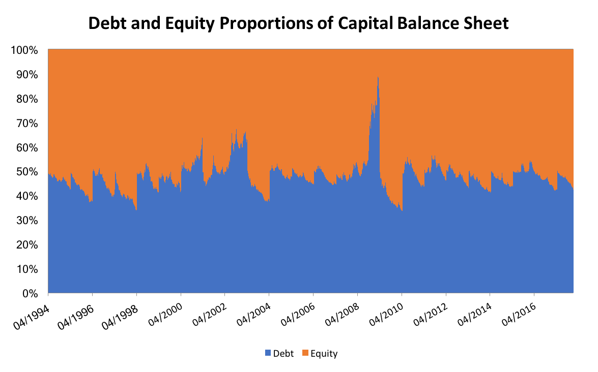
Source: CSI. Calculations by Newfound Research. Assumes portfolio applies 100% notional leverage applied to SPDR S&P 500 ETF (“SPY”) at inception of ETF and reset every 252-days thereafter. Assumes zero cost of leverage.

Note that in 2008, the debt proportion of our balance sheet spiked up to nearly 90% of our capital. What happened? This is reset timing risk. On 4/2008, the portfolio reset, borrowing $92,574 against our equity of $92,574. Over the next year, the market fell approximately 39%. Our total assets tumbled from $185,148 to $114,753 and we still owed the initial $92,574 we borrowed. Thus, our actual equity over this period fell an astounding -76.7%.

(It is worth pointing out that if we had considered a “never reset” portfolio that started on 4/2008, we’d have the same result.)

Frequent readers of our commentary may be wondering, “can this reset timing risk be controlled with overlapping portfolios just like other timing risks?” Yes … ish. On the one hand, there is not a whole lot we can do about the drawdown itself: 100% notional leverage plus a 37% drawdown means you’re going to have a bad time. Where overlapping portfolios can help is in ensuring that resets do not necessarily occur at the worst possible point (e.g. the bottom of the drawdown) and lock in losses.

As a general rule, we probably don’t want to apply N-times exposure over a time frame an asset class can experience a return of -1/N%. For example, if we want 2x equity exposure, we want to make sure we reset our leverage exposure well before equities have a chance to lose 50% (1/2). Similarly, if we want 3x exposure, we need to reset well before we can lose 33.3% (1/3).

So, Are They Evil or What?

We would argue that volatility decay takes the blame when it is not actually the culprit. Volatility decay is nothing more than the math of compounding returns: it happens whether you are levered or not.

The danger of most levered ETFs is more easily explained. If I told you I was going to take your investment, use it as collateral to gain 100% notional exposure to equities, and then invest that collateral in equities as well – an asset class than can easily lose 50% –what would you say? When put that way, it sounds a little nuts. It really isn’t much more complicated than that.

The reset effect really just introduces a few more nuanced wrinkles. The more frequently we reset, the less risk we run of going bust, as we take risk off the table as our debt-to-equity ratio climbs. That’s how we can avoid complete ruin with 100% leverage in an asset class that falls more than 50%.

On the other hand, the more frequently we reset, the closer we keep the portfolio to the target volatility level, increasing the drag from short-term mean reversion.