
By Justin Sibears, Newfound Research
We often compare portfolio construction to cooking. There are two equally important elements: the ingredients and the recipe. The ingredients are the signals that are used to select investments. The recipe is the set of rules used to transform those signals into portfolio allocations.
When it comes to factor investing, it seems that the signals oftentimes get all the attention. Investors struggle with whether incorporating factor-based strategies is worth it, argue over which are the premier factors, debate whether factors can be timed or not, and fret about premiums being driven towards zero as acceptance of factor-based strategies increases.
In all of this (admittedly an interesting debate), the importance of the recipe – i.e. how we move from a factor score to an actual strategy – is often lost.
Let’s use the momentum factor as an example. What decisions do we need to make to build a momentum portfolio?
First, we need to decide how to measure momentum. The simplest and most traditional approach would just be to use trailing total return. However, there are many other ways to measure momentum. We could use risk-adjusted momentum (i.e. looking at trailing Sharpe Ratios instead of trailing returns). We could use idiosyncratic momentum (i.e. measuring trailing returns after stripping out the stock’s exposure to the broad market). We could use a regression on past prices to estimate the stock’s trend. We could smooth prices using various moving averages. We could diversify by blending multiple signals together.
We also need to decide over how long of a period we want to measure momentum. Do we want to use 12 months? 9 months? 6 months? Do we want to skip to the most recent month to account for mean reversion as is common in the academic literature or include it?
Do want to rebalance weekly, monthly, quarterly, or at some other interval?
How concentrated do we want the portfolio to be? Do we choose the 30 stocks with the highest momentum? 50 stocks? 100 stocks?
How will the stocks be weighted? We could market-cap weight the holdings. We could equal-weight the holdings. We could allocate in proportion to each stock’s momentum by giving the highest allocation to the stocks with the most momentum.
If we wanted to get really fancy we could run some type of optimization like equal-risk contribution, mean-variance optimization, or minimum volatility.
If we go this route, then we really open Pandora’s box. We now need to decide how to estimate our parameters (means, volatility, and correlations). Do we use historical data? If so, how much? What measures do we use? How do we account for estimation risk?
Do we care about controlling for other risk factors, like sector risk? If not, we may let the portfolio be sector unconstrained and therefore let the sector exposures just fall out of the stock selection. If yes, we need to decide how to control it. Do we force the portfolio to be sector neutral (i.e. have the same sector weights as the market)? Are we comfortable with a middle ground, where sector weights are allowed to drift from market-cap sector weights, but only by some pre-specified amount? If we want to go this route, how loose or tight do we set those thresholds?
We could go on and on and on. The degree of potential customization of the recipe is largely limitless. In the ramblings above, we mentioned at least six dimensions of customization for a momentum strategy:
- Momentum measure
- Lookback period
- Rebalance frequency
- Concentration
- Weighting Scheme
- Sector Constraints
If these were the only six dimensions and there were only ten choices per dimension, there would be a whopping 1,000,000 potential variations of the momentum strategy!
Illustrating the Impact of the Portfolio Construction Recipe
To illustrate the impact that these choices can have on returns, we conducted a simple experiment. Our investment universe consists of the 200 largest holdings in the SPDR S&P 500 ETF (ticker: SPY)[1]. Using this universe, we create 1,080 different momentum portfolios by varying the construction rules (5 momentum measures x 4 lookback periods x 3 rebalance frequencies x 3 levels of portfolio concentration x 3 weighting schemes x 2 methods of dealing with sector risk[2]).
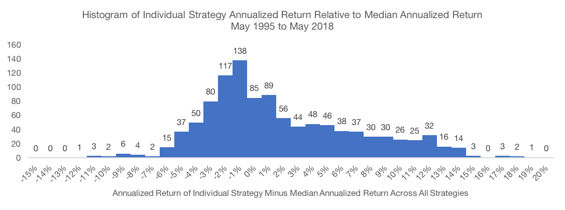
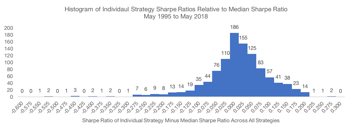
As a quick note, since we are only interested in exploring dispersion across strategies, all performance statistics presented are normalized by subtracting the median for that metric across all 1,080 strategies. For example, an annualized return of +5.0% means that a strategy outperformed the median by 5.0% per year. Similarly, a Sharpe Ratio of -0.10 simply says that the strategy’s Sharpe Ratio was 0.10 lower than the median Sharpe Ratio across all 1,080 strategies.
The dispersion of full period performance statistics is quite large. On a raw return basis, the worst performing strategy underperformed the median by 12.0% annualized while the best performing strategy outperformed the median by 18.0% annualized. A difference of more than 30% per year between the best and worst strategy is certainly nothing to sneeze at. Even if we ignore the tails of the return distribution, the dispersion remains very evident. The 95% confidence interval is -5.5% to +11.5%. The standard deviation of annualized returns across the strategies tested is 5.3%.
The results are very similar if we change focus to risk-adjusted returns using the Sharpe Ratio. The worst strategy on a risk-adjusted basis has a Sharpe Ratio 0.57 below the median, while the best strategy’s Sharpe Ratio is 0.27 above the median. The 95% confidence interval is -0.18 to +0.14 and the standard deviation of Sharpe Ratio relative to the median is 0.10.
![]()
Data Source: CSI and SPDR. Calculations by Newfound Research. Data analysis starts in May 1995 as that is when all portfolios could calibrate given available price data. Returns are hypothetical and backtested and do not reflect any strategy managed by Newfound Research. Returns include the reinvestment of dividends. The strategies all were constructed with explicit hindsight bias as the universe consists of the 200 largest stocks in the SPDR S&P 500 ETF (ticker: SPY) as of May 2018. Past performance does not guarantee future results.
Data Source: CSI and SPDR. Calculations by Newfound Research. Data analysis starts in May 1995 as that is when all portfolios could calibrate given available price data. Returns are hypothetical and backtested and do not reflect any strategy managed by Newfound Research. Returns include the reinvestment of dividends. The strategies all were constructed with explicit hindsight bias as the universe consists of the 200 largest stocks in the SPDR S&P 500 ETF (ticker: SPY) as of May 2018. Past performance does not guarantee future results.
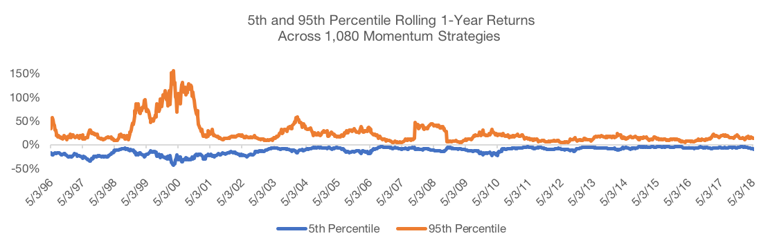
While the dispersion of full period results is interesting, what we really want to focus on is the dispersion in returns over shorter time horizons because these are the differences that fuel many behavioral biases. To do so, we calculate rolling one-year returns for each of the strategies. We then rank these returns across all strategies at each point in time and then plot the 95% confidence interval. Again, all returns are normalized by subtracting the median return at each point in time.
Data Source: CSI and SPDR. Calculations by Newfound Research. Data analysis starts in May 1995 as that is when all portfolios could calibrate given available price data. Returns are hypothetical and backtested and do not reflect any strategy managed by Newfound Research. Returns include the reinvestment of dividends. The strategies all were constructed with explicit hindsight bias as the universe consists of the 200 largest stocks in the SPDR S&P 500 ETF (ticker: SPY) as of May 2018. Past performance does not guarantee future results.
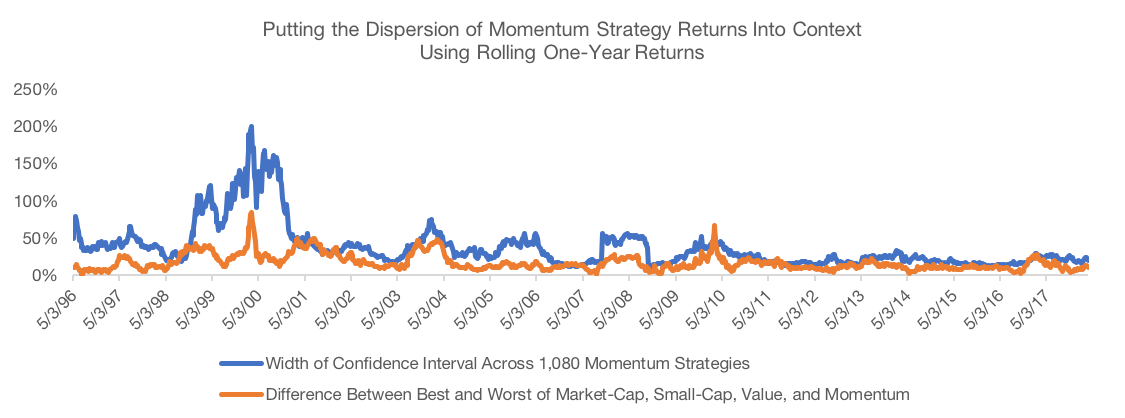
To put this dispersion into context, we use Fama-French data to calculate rolling one-year returns for four long-only equity portfolios: a market-cap weighted portfolio, a value portfolio (top 30% of universe by book-to-price), a momentum portfolio (top 30% by 12-month trailing return skipping the most recent month), and a small-cap portfolios (bottom 30% of the universe by market-cap). We then calculate the difference between the best and worst performing of these strategies. We compare this quantity to the width of the 95% confidence interval over our 1,080 momentum strategies.
We find that more than 90% of the time, the variation across the different momentum strategies is greater than the variation across the factors. In other words, whether momentum beats value or momentum beats size can be very, very dependent on how each of the individual factor portfolios is constructed.
Let that sink in for a minute. In the short-term, it is entirely possible that one approach to capturing momentum outperforms other factors like value and size while another implementation of momentum underperforms.
Data Source: CSI, SPDR, Fama French Data Library. Calculations by Newfound Research. Data analysis starts in May 1995 as that is when all portfolios could calibrate given available price data. Returns are hypothetical and backtested and do not reflect any strategy managed by Newfound Research. Returns include the reinvestment of dividends. The strategies all were constructed with explicit hindsight bias as the universe consists of the 200 largest stocks in the SPDR S&P 500 ETF (ticker: SPY) as of May 2018. Past performance does not guarantee future results.
In past speaking engagements, we’ve argued that successful factor investing can be boiled down to the following three Warren Buffett quotes:
- “Risk comes from not knowing what you are doing.” → Takeaway: Know what you own. Understand not only the factors being employed, but also how the portfolio is constructed.
- “You don’t need to be a rocket scientist. Investing is not a game where the guy with the 160 IQ beats the guy with 130 IQ.” → Takeaway: Know why you own it. Data should never trump insight, but theories must be supported by the data.
- “No matter how great the talents or efforts, some things just take time. You can’t produce a baby in one month by getting nine women pregnant.” Takeaway → Commit to owning it. Factor premiums vary over time. All factors go through periods of prolonged underperformance. The biggest benefits will accrue to those investors with the discipline to stay committed through these difficult periods. Put differently, weak hands that “fold” will pass to premium to strong hands that “hold.”
We think the types of results illustrated in this commentary have important implications for all three of these aspects of factor investing.
Know What You Own
Once you’ve decided what type of exposure you are interested in adding to a portfolio, the first step of due diligence is understanding the investment process. In our minds, one of the biggest advantages of index-based ETFs is that there is no guessing when it comes to understanding the investment process. We don’t have to rely on manager interviews and presentations. We don’t have to worry that manager will change his or her investment process when the going gets tough. Understanding the investment process is as simple as digging into to the index methodology.
Take the following four momentum ETFs as examples:
- iShares Edge MSCI USA Momentum ETF (ticker: MTUM, tracks the MSCI USA Momentum Index)
- SPDR Russell 1000 Momentum Focus ETF (ticker: ONEO, tracks the Russell 1000 Momentum Focused Factor Index)
- Fidelity Momentum Factor ETF (ticker: FDMO, tracks the Fidelity U.S. Momentum Factor Index)
- JPMorgan U.S. Momentum Factor ETF (ticker: JMOM, tracks the JPMorgan US Momentum Factor Index)
Summary of Index Methodology
| MTUM | ONEO | FDMO | JMOM | |
| Factor | Momentum | Momentum | Momentum | Momentum |
| Universe | MSCI USA Index (85% free float of U.S. market, currently has 631 constituents). | Russell 1000 | Largest 1000 stocks based on market-capitalization | Russell 1000 |
| Measure | Blend of trailing 12-month and 6-month risk-adjusted price return in excess of risk-free rate and skipping the most recent month. Currently has 125 securities (approximately 20% of the stocks in the universe). | 12-Month Total Return (skipping most recent month). The process also considers value (Composite of cash flow yield, earnings yield, and sales-to-price.), quality (Composite of profitability and leverage. Profitability is a blend of return on assets, change in asset turnover, and accruals. Leverage is the ratio of operating cash flow to total debt), and size (natural logarithm of market-capitalization). | Blended score with 35% weight on 12-month total return (skipping most recent month), 35% on volatility-adjusted 12-month total return (skipping most recent month, monthly returns used to calculate volatility), 15% on 12-month earnings surprise (EPS estimate from 12-months ago to actual EPS), and 15% on 12-month average short interest. Composite scores are size-adjusted to minimize any size bias. | 12-Month Total Return Divided by Volatility (volatility measured using 1 year of daily returns) |
| Rebalance Frequency | Semi-Annual with ability for more frequent rebalances depending on volatility of the index. | Semi-Annual | Quarterly | Quarterly |
| Concentration | Dependent on the number of securities in the parent index and the market-cap distribution of securities. | No explicit concentration, although there is a minimum position size. Currently holds positions in approximately 88% of the companies in the universe. | Top decile (10%) within sectors with more than 100 securities. Top quintile (20%) within sectors with 25 to 100 securities. Top tercile (33%) for sectors with less than 25 securities. Currently holds positions in approximately 13% of the stocks in the universe. | No defined concentration. Currently holds positions in approximately 27% of the stocks in the universe. |
| Weighting Methodology | Multiply momentum score by market-capitalization. | “Tilt-tilt” methodology multiplies the factor scores for quality, value, size, and momentum. | Market-cap within each sector plus an equal overweight adjustment that is applied equally to all constituents within that sector. | Weights to companies in industries that are under the required allocation are increased in an iterative fashion starting with the stock with the highest momentum. Similarly, weights to companies in industries that are over the required allocation are decreased in an iterative fashion starting with the stock with the worst momentum. There is then a set of rules that (i) ensures that the total amount invested equals 100% of the portfolio and (ii) allows for rebalancing from the stocks with the worst momentum to the stocks with the best momentum. |
| Sector Constraints | N/A | Lower and upper bounds applied by industries, but are not relative to the market-cap of each industry. | Sector neutral relative to investment universe | Industry neutral relative to Russell 1000 |
| Other Constraints | 5% position limit. | Maximum position limit tied to capacity/liquidity. | N/A | Individual position limits are a function of market-cap and liquidity with a hard limit of 2%. |
| Other Notes | Apply buffer rules to manage turnover. | N/A | N/A | The index actively considers liquidity in deciding how large of trades are required at each rebalance. |
Source: FTSE, MSCI, Fidelity, Data as of May 18, 2018
We immediately see the diversity in investment processes across the different strategies. None of the strategies measure momentum the exact same way, let alone have much overlap in the many dimensions of the construction rules like sector limits, weighting methodology, etc.
These differences are abundantly clear when we examine the top holdings, sector holdings, and holdings overlap.
