

Top Ten Holdings by ETF
| MTUM | ONEO | FDMO | JMOM |
| Microsoft (5.1%) | Micron (1.0%) | Apple (4.4%) | Apple (2.1%) |
| Amazon (5.0%) | Lear (0.9%) | Microsoft (3.5%) | Amazon (2.0%) |
| JPMorgan (4.9%) | Best Buy (0.8%) | Amazon (3.0%) | Microsoft (2.0%) |
| Intel (4.6%) | Aptiv (0.8%) | Facebook (2.4%) | Facebook (2.0%) |
| Boeing (4.5%) | Baxter (0.8%) | JPMorgan (2.1%) | Visa (1.8%) |
| Bank of America (4.5%) | XPO Logistics (0.7%) | Berkshire Hathaway (2.0%) | Google (1.8%) |
| Cisco (4.1%) | Corning (0.6%) | Johnson & Johnson (2.0%) | UnitedHealth (1.7%) |
| Mastercard (3.6%) | Michael Kors (0.6%) | UnitedHealth (1.7%) | Home Depot (1.6%) |
| Abbvie (3.3%) | Valero (0.5%) | Visa (1.7%) | Johnson & Johnson (1.6%) |
| Visa (3.2%) | Spirit AeroSystems (0.5%) | Mastercard (1.5%) | Boeing (1.5%) |
Source: JPMorgan, Fidelity, iShares, and SPDR as of May 18, 2018.
![]()
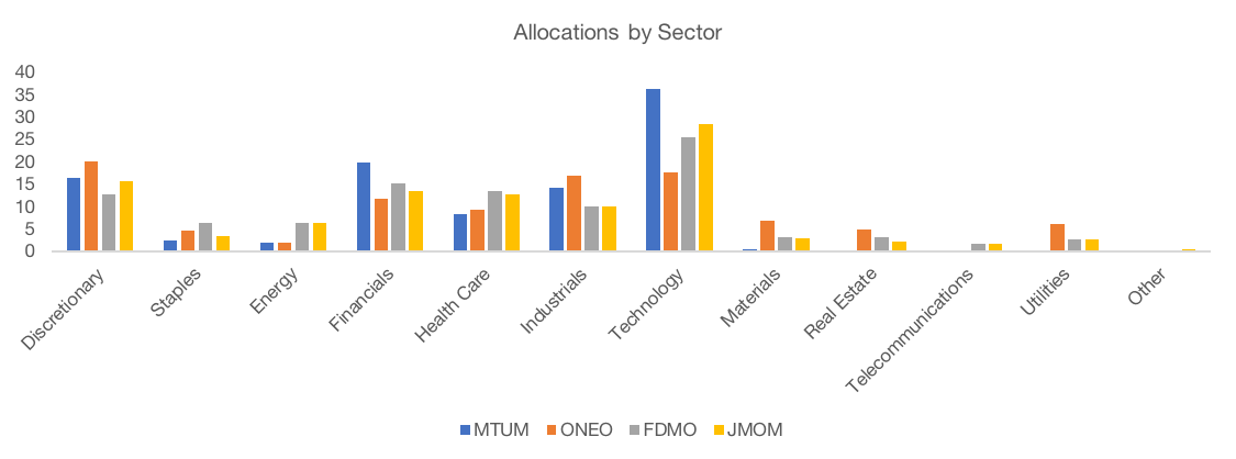
Source: Bloomberg
Holdings Overlap
| MTUM | ONEO | FDMO | JMOM | |
| MTUM | 100% | 15% | 36% | 34% |
| ONEO | 100% | 17% | 34% | |
| FDMO | 100% | 50% | ||
| JMOM | 100% |
Source: Bloomberg
Know Why You Own It
Knowing why you own is the second step in the diligence process. Once we understand how the strategy works by digging into the index methodology, our work must turn to understanding the why behind the design. The biggest due diligence implication of our study of different iterations of momentum strategies is that due diligence does not begin and end with finding the right factors. Performing due diligence on the portfolio construction process that translates the factor signals into actual allocations is just as crucial.
Just because a strategy or index touts itself as harvesting one of the handful of factors that are supported by both sound economic theory and broad out-of-sample performance (e.g. value, momentum, trend, carry) does not mean that it is immune from data mining.
In fact, it’s even entirely possible that a factor that has exhibited no long-term efficacy can be made to appear statistically significant just by over-optimizing the portfolio construction rules using the same signals.
Some techniques/rules of thumb that we adhere to when performing this type of diligence are:
- Holding all else equal, simpler is better. Simpler processes have fewer degrees of freedom and therefore are less susceptible to being data mined.
- Ask “Why?” In the first item above, the “holding all else equal” is just as important as the “simpler is better.” Perhaps the simplest momentum strategy would just constantly trade into the single stock with the highest momentum. Such a strategy, while simple, happens to be foolish. Complexity has its place, if used with purpose.Key elements of the recipe should be held to the same standard that we hold the factors themselves to. Namely, we should look for construction rules that are backed by both empirical evidence; preferably across asset classes, geographies, and time frames; and sound theory.Take rebalance frequency as an example. In a world with no transaction costs, it may make sense to rebalance continuously so as to maximize the desired factor exposure at each point in time. Of course, this type of construction, especially for a higher turnover factor like momentum, may incur such high transaction costs that the amount of excess return may be materially or even completely eliminated.
- Ask to see sensitivity analysis across parameters. With index-based strategies, it should be relatively simple for the index or ETF provider to provide insight into how varying a particular parameter would have impacted risk/return in the historical data. As an example, consider a strategy that constrains turnover to X% at each rebalance date. We think it’s entirely reasonable to ask how overall turnover and performance would be impacted by varying that parameters above and below X%. It would be worth noting if X% happened to be an isolated optimal value based on historical performance. Such a result for one parameter would not necessarily be overly concerning, but if we saw the same result across a number of parameters then our data mining alarm bells should be ringing.
- Embrace process diversification. One elegant way to address the idiosyncratic risk across strategies when we don’t have a strong, evidence-based view as to whether one construction is better or worse than another is simply to diversify across parameters. In our simulated momentum strategies, we find that an equal weighted blend of all 1,080 strategies has a better raw and risk-adjusted return than the median of the individual strategies. We employ this type of approach in our tactical strategies where we prefer a monthly rebalance, but are concerned with timing luck (i.e. tracking error that can arise between monthly rebalanced strategies that rebalance at different times during the month). To address this risk, we manage a number of sub-portfolios that are each rebalanced at a different time during the month.
- Beware the magic number. “Magic numbers” are parameters that are unlikely to be chosen by design and rather suggest that the process has been optimized over the historical data set. For example, say there was a value ETF that used three different valuation metrics: price-to-earnings, price-to-book, and price-to-sales. The underlying index creates a composite value score for each stock according to the following formula: Value Score = 0.243 * Normalized P/E + 0.619 * Normalized P/B + 0.138 * Normalized P/S.This is an immediate red flag. It’s unlikely that such a specific formula was derived by anything other than analysis of the historical data and that over-optimization, whether intentional or accidental, has infiltrated the strategy design.
On a related note, there is evidence in our minds that data mining is occurring. For example. “Live from Newport Beach. It’s Smart Beta!”, an August 2017 piece from Feifei Li and John West at Research Affiliates, is a must read for those looking to get into the factor investing game. In the article, the authors examine 125 U.S. equity smart beta or indices that are tracked by ETFs. They conclude: “We find that prior to launch the indices tend to have superior performance relative to a market-capitalization-weighted benchmark, with outperformance peaking about six months ahead of the launch date. The outperformance seems to be extremely strong over the three-year period ahead of the launch. After the indices officially launch, however, their performance relative to the S&P 500 Index appears to hover around the base line, exhibiting virtually none of the outperformance demonstrated before they were live.”
The punchline is summed up nicely in the following chart:
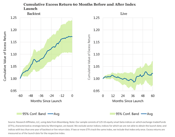
There are a few ways you could interpret this data.
You could conclude that factor investing is fundamentally broken. It may have worked historically in a backtest but has not actually played out so well for ETF investors in the real world, whether because the factors themselves were data mined, increased usage as driven premiums to zero, or some other reason. We don’t believe this is the case. We’d be more worried about this if the factor products being launched largely reflected new factors that had yet to be proven through significant out-of-sample study. Yet, most launches have tended to stick to the factors that check all the right boxes like momentum, value, and low volatility.
Rather, we hypothesize that two things are going on here. First, index providers and ETF manufacturers are not immune to chasing performance. At the end of the day, asset management as a business is about sales. Selling an asset class or strategy that has outperformed recently is infinitely easier than selling one that has underperformed. When the strategies inevitably mean revert, as long-term performance tends to, you get results like those seen in the Research Affiliates piece. Looking at live performance between 60 months and 120 months may be a clearer indicator of this fact.
Second, there may be some data mining going on at the recipe level. Let’s return to our 1,080 momentum strategies for a second. Assume that these represent different potential indices that may be tracked by new ETFs. Each week, we’ll assume that one new momentum ETF is launched. This new ETF will track an index that was randomly chosen from the top 5% of the 1,080-index universe based on trailing five-year Sharpe Ratio[3]. In other words, performance chasing has infected the product development process. After performing this simulation, we plot the average 1-year Sharpe Ratio in the 5-years before and after product launch.
Unsurprisingly, we see a similar situation in our simulation as the actual data from the Research Affiliates. Performance is strong relative to the entire universe of momentum strategies pre-launch (by definition since the “launched” strategies are picked from the group of the best historical performers), but this outperformance erodes in the years after launch.
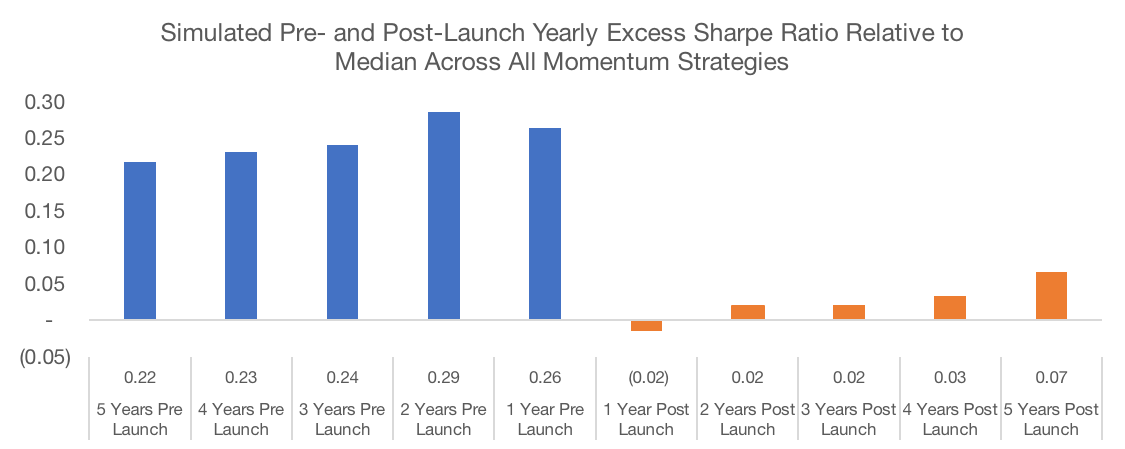
Data Source: CSI and SPDR. Calculations by Newfound Research. Data analysis starts in May 1995 as that is when all portfolios could calibrate given available price data. Returns are hypothetical and backtested and do not reflect any strategy managed by Newfound Research. Returns include the reinvestment of dividends. The strategies all were constructed with explicit hindsight bias as the universe consists of the 200 largest stocks in the SPDR S&P 500 ETF (ticker: SPY) as of May 2018. Past performance does not guarantee future results.
Commit to Owning It (No Pain, No Premium)
Factor investing is not a painless process. Underperformance for any individual factor strategy, even over a five-year period, should not be alarming in isolation. In fact, the ability to weather prolonged periods of underperformance has historically been a necessary condition for capturing the long-term benefits of factor investing. Going back to the 1930s, all four factors presented below (size, value, momentum, and low beta) show significant positive annualized excess returns, but experience drawdowns that are comparable in duration and magnitude to those seen in the equity market as a whole.
No Pain, No Premium → The Experience of a Factor Investor
| Market (MKT) |
Size (SMB) |
Value (HML) |
Momentum (UMD) |
Low Beta (BAB) |
|
| Annualized Excess Return | 6.8% | 1.8% | 3.5% | 7.3% | 7.9% |
| Annualized Volatility | 18.3% | 10.4% | 11.7% | 15.7% | 11.0% |
| Maximum Drawdown | 54.3% | 54.5% | 38.9% | 58.3% | 52.9% |
| Longest Drawdown | 12.4 Years | 34.7 Years | 11.0 Years | 9.3 Years | 6.8 Years |
| Ulcer Index | 17.2 | 24.9 | 12.5 | 17.5 | 12.0 |
Data Source: AQR. Calculations by Newfound Research. Data covers the period from 1935 to 2018. Returns are hypothetical and do not reflect any strategy managed by Newfound Research. Returns include the reinvestment of dividends. Past performance does not guarantee future results.
The immense tracking error that can be experienced even across strategies utilizing the same general factor creates even more opportunities for doubt to creep in and commitment to erode.
On multiple occasions, we’ve participated on panels related to factor-investing and been something along the lines of “Is factor investing worth it?” Our answer is a resounding yes, with one caveat. There needs to be long-term commitment. If a factor or strategy will be sold a year from now if it has underperformed, that investor’s experience is much less likely to be positive.
In our momentum strategy simulations, we see that performance chasing does not work. There is almost no relationship between trailing 1-year Sharpe Ratios and forward 1-year Sharpe Ratios. When we expand the performance measurement interval to three and five years, we see clear evidence of mean reversion. High past Sharpe Ratios tend to predict low future Sharpe Ratios and vice versa. Buyer beware that strong recent track records alone should provide little comfort as to future expectations.
| Correlation | OLS Beta | R^2 | |
| Trailing 1-Year Sharpe vs. Forward 1-Year Sharpe | 0.07 | 0.07 | 0.01 |
| Trailing 3-Year Sharpe vs. Forward 3-Year Sharpe | -0.48 | -0.49 | 0.23 |
| Trailing 5-Year Sharpe vs. Forward 5-Year Sharpe | -0.61 | -0.78 | 0.37 |
Data Source: CSI and SPDR. Calculations by Newfound Research. Data analysis starts in May 1995 as that is when all portfolios could calibrate given available price data. Returns are hypothetical and backtested and do not reflect any strategy managed by Newfound Research. Returns include the reinvestment of dividends. The strategies all were constructed with explicit hindsight bias as the universe consists of the 200 largest stocks in the SPDR S&P 500 ETF (ticker: SPY) as of May 2018. Past performance does not guarantee future results.
Conclusion
Portfolio construction is a lot like cooking. There are two equally important elements: the ingredients and the recipe. The ingredients are the signals that are used to select investments. The recipe is the set of rules used to transform those signals into portfolio allocations.
In factor investing, the signals (e.g., value, momentum, carry) often get all the attention and the importance of the recipe – how these signals are actually transformed into portfolio construction – often gets lost. Designing a recipe requires making decisions like how often to rebalance, how to weight holdings, and how to blend signals (when multiple signals are used).
Even portfolios that use the same core factor can experience significant performance dispersion due to recipe differences.
This dispersion has two main implications for factor investors. First, dispersion creates the opportunity for data mining. To combat this, diligence efforts must focus as much on the construction process as they do on the factors themselves.
Second, dispersion makes short-term underperformance inevitable. Potential dispersion is so large due to recipe differences that it is entirely plausible that one momentum portfolio, as an example, could outperform value while another underperforms. Users of factor strategies should resist the urge to chase performance, especially over 3- to 5-year investment horizons.
[1] Because we use the current top 200 holdings, we are knowingly introducing hindsight bias into the portfolio process. Overall, we would expect a portfolio consisting of SPY’s current top holdings to have strong past performance, otherwise many of the companies may not be in the top 200 by market-cap today. We are fine with this because our goal is to illustrate the how much return dispersion can be created through the selection of the portfolio construction rules. However, due to the hindsight bias, the results should not be used to draw conclusions as to how any of these strategies in particular, or the momentum factor in general, would have performed historically or how they may perform going forward, especially in comparison to the broad market.
[2] Momentum measures are trailing total return, trailing total return skipping the most recent month, risk-adjusted trailing total return, OLS estimate of the trend, and a Kalman filter. The lookbacks are 3 months, 6 months, 9, months, and 12 months. The rebalance frequencies are weekly, monthly, and quarterly. In the most concentrated portfolio we pick the top 10% of stocks by momentum. In the least concentrated portfolio we pick the top 50% of stocks by momentum. The middle level of concentration picks the top 25% of stocks by momentum. The weighting schemes are equal-weighted, rank-weighted, and score-weighted. We consider both sector constrained (sector weights equal to market-cap sector weights) and sector unconstrained strategies.
[3] We randomly select from the top 5% instead of simply choosing the best strategies to try to ensure that there is some diversity among the strategies. Choosing the top strategy would probably lead to a lot of overlap. We think this is a more realistic representation of reality since it does seem that product manufacturers and index providers seek to differentiate their strategies from others in the market.