
![]() By Justin Sibears, Newfound Research
By Justin Sibears, Newfound Research
Generally speaking, risk parity portfolios attempt to diversify across asset classes and strategies by risk contribution as opposed to dollar allocation. The classic argument for risk parity typically begins by noting that many traditional portfolios (e.g. the 60/40 or “balanced” portfolio) are dominated by equity risk. A risk parity approach, on the other hand, can lead to portfolios that are more appropriately diversified across risk factors.
Dollar Allocation vs. Risk Allocation for Equal Risk Contribution Portfolio of S&P 500 and Barclays Aggregate Bond
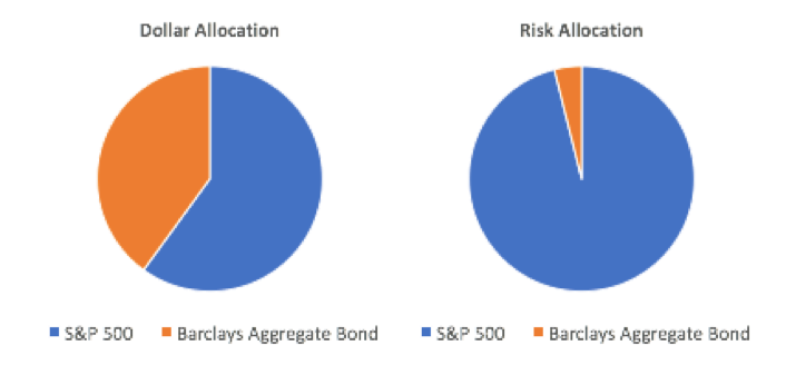
Data Source: CSI, Calculations by Newfound Research. The S&P 500 is represented by the SPDR S&P 500 ETF and the Barclays Aggregate Bond Index is represented by the iShares Core U.S. Aggregate Bond ETF. Data for the risk calculation covers the period from September 2003 to October 2017. Past performance does not guarantee future results.
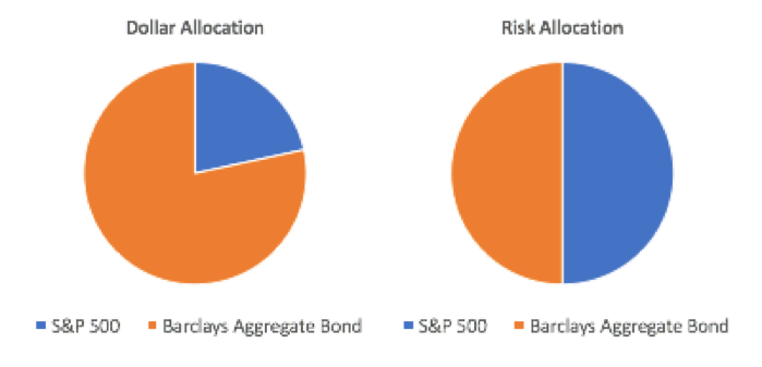
Data Source: CSI, Calculations by Newfound Research. The S&P 500 is represented by the SPDR S&P 500 ETF and the Barclays Aggregate Bond Index is represented by the iShares Core U.S. Aggregate Bond ETF. Data for the risk calculation covers the period from September 2003 to October 2017. Past performance does not guarantee future results.
Risk parity checks off all of our main boxes for strategy selection. It is backed by both strong empirical evidence and sound economic theory. Just as importantly, risk parity can be implemented through a simple, transparent, and systematic investment process.
When constructing a risk parity portfolio, there are a number of questions that need to be answered, including:
- What is my investment universe?
- How am I going to measure risk?
- How do I account for correlations?
- Am I willing to use leverage? If so, how do I set my total notional exposure? Or framed differently, what is my target volatility?
- How do I account for real world complexities like trading, transaction costs, and taxes?
With respect to question #2, many practitioners use historical data to calculate risk. When using the historical approach, we have to select both the risk metric(s) to use and the period length(s) over which to measure the selected metrics. For example, Salient’s risk parity white paper uses rolling two-year periods of daily returns to calculate volatilities and correlations.
In this commentary, we are going to explore the importance of the lookback period. Namely, does the length of lookback period matter? And if it does, are we better off using as much data as possible (i.e. long lookback periods) or focusing on just the more recent past (i.e. short lookback periods).
Building a Simple Risk Parity Strategy
To answer these questions, we have to build a risk parity strategy. For simplicity, we will use ETFs for our analysis even though most real world risk parity strategies implement via futures. We consider ETFs in four asset classes:
- Equities
- Fixed Income
- Real Assets (Commodities and TIPs)
- Credit/Currency (investment grade and high yield corporate bonds, dollar-denominated emerging market bonds, local currency emerging market bonds).
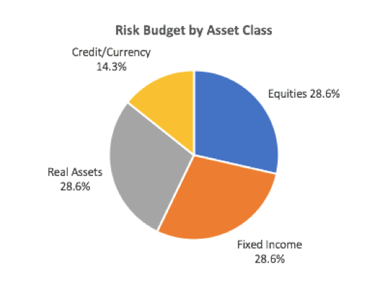
Our target risk allocation is presented in the following pie chart. Within each asset class, we distribute the risk budget either equally or by market-capitalization. For chart readability, we only show the risk budget at the asset class level (full risk budget targets are available on request).
Note that the credit/currency bucket gets half the risk budget of the other three asset classes. This is a byproduct of using ETFs instead of futures contracts. In a real-life implementation, we could truly isolate the credit and currency exposure by using credit default swaps and currency forwards, respectively. However, with ETFs we are forced to get the exposure via bonds. These bonds have embedded interest rate risk in additional to the credit/currency components. Therefore, we lower the risk budget for this bucket to avoid being too structurally overweight interest rate risk.
We examined lookback periods ranging from 63 trading days (approximately one quarter of data) to 6300 trading days (25 years). For each lookback period, we computed two hypothetical portfolios. One portfolio was managed using simple volatilities and correlations, while the other used exponentially-weighted volatilities and correlations. The decay factor for the exponentially-weighted metrics were set so that the half-life was equal to half of the lookback period[2].
For each combination of lookback period (1 quarter to 25 years) and calculation type (simple or exponentially-weighted), we created a hypothetical portfolio. Each of these portfolios was rebalanced monthly using the following process:
- Estimate volatilities and correlations using the given lookback period and calculation type. Volatilities were estimated using daily data. Correlations were estimated using weekly data.
- Compute the portfolio weights such that the risk contribution of each positon equals the target risk budget. We normalize these weights so that they sum to 1.
- Scale the portfolio weights to a total notional value such that we target a volatility of 10%.
Evaluating the Allocations
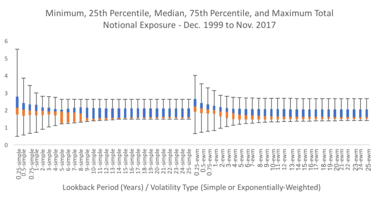
From an allocation perspective, the results aren’t all that surprising. Below, we present a box-and-whisker plot for the total notional exposure though time. The data points represented are the minimum, 25th percentile, median, 75thpercentile, and maximum total exposure. We see more variation in allocations for shorter lookback periods. For example, a lookback period of 63 trading days – or one quarter- leads to total notional exposure that ranges from a low of 47% to a high of 552% when simple volatilities are used. On the other hand, the range is only 137% to 263% for a 10-year lookback period.
We also see that median exposure tends to decline as the lookback period is expanded. The median exposure is 214% for the 63-day lookback and 149% for the 10-year lookback.
A natural byproduct of more reactive allocations is higher turnover. We do see that turnover declines very quickly as the lookback period is expanded. When using simple volatility, annualized turnover is 337% when one quarter of data is used, 155% when two quarters are used, 107% when three quarters are used, and 79% when 1 year is used. Turnover drops below 50% once at least two years of data is incorporated.
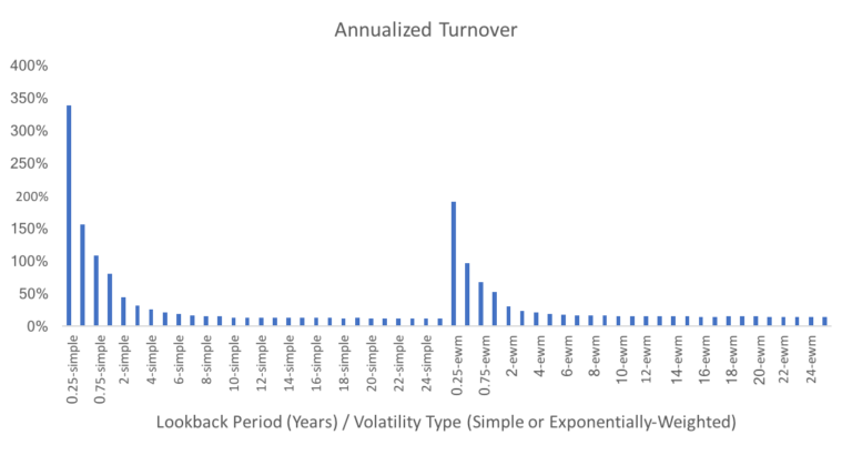
Data Source: CSI. Calculations by Newfound Research. Risk parity indices are backtested and hypothetical and do not reflect any strategies managed historically by Newfound Research. Results cover the period from December 1999 to November 2017. Past performance does not guarantee future results.
In terms of asset classes, we see the average allocation to real assets and fixed income increasing and the average allocation to equity and credit/currency decreasing as the lookback period is extended. This makes sense given the market path during the period studied. The longer lookback periods have more “memory” of the volatility spike experienced by many “risk-on” asset classes during the global financial crisis. These asset classes are therefore penalized for 2007-09 even during the more benign risk environment of the current equity bull market. The trends are similar, but less pronounced, when we use exponentially-weighted statistics.
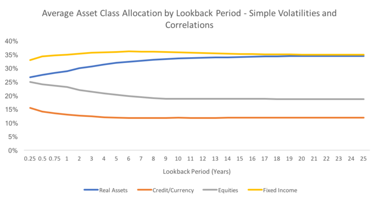
Data Source: CSI. Calculations by Newfound Research. Risk parity indices are backtested and hypothetical and do not reflect any strategies managed historically by Newfound Research. Results cover the period from December 1999 to November 2017. Past performance does not guarantee future results.
Evaluating Performance
The Sharpe Ratios generated by the various strategies are remarkably stable. They are all clustered between a minimum of 0.61 (two-year lookback, simple volatility) and 0.72 (1-quarter lookback, exponentially-weighted volatility).
When simple volatilities are used, Sharpe Ratios initially decline as the lookback period is expanded through two years. From two years to five years, Sharpe Ratios recover before stabilizing for 5+ years of data at a level that is almost identical to the Sharpe Ratio for a one-quarter lookback.
Using exponentially-weighted statistics seems to eliminate much of this noise since, excluding the one-quarter lookback, all of the exponentially-weighted Sharpe Ratios are between 0.676 and 0.681.
Using the Sharpe Ratio comparison methodology outlined in Opdyke (2007)[3], we were able to verify that these Sharpe Ratio differences are not statistically significant when we account for skew and kurtosis.
