As we have discussed in our prior articles in this ETF Strategist series (Article 1, Article 2, Article 3), Risk-Managed Investing (RMI) is the attempt to embed downside risk management directly into an equity investment.
One feature of a successful RMI strategy is the reduction in volatility compared to a corresponding traditional equity investment, i.e., one that does not possess an explicit risk-management element. Volatility reduction has well-known qualitative benefits, including enhancing investor peace of mind and helping exceptionally skittish individuals overcome their fear and hold the appropriate amount of equities in their portfolios.
RMI’s volatility reduction can also deliver quantitative benefits, and these may be less obvious or appreciated, but they can be explicitly calibrated. Let’s explore two such benefits, the reduction in “volatility drag” and the mitigation of “sequence risk.”
Volatility drag can be illustrated by the following simple example, in which we compare a rock-steady 8% annual return with a fairly erratic return stream that happens to average 9%.
The 9%-return portfolio results in lower ending wealth than the 8%-return portfolio! It seems clear from this that there is demonstrable economic value in stability of returns. This can be quantified more generally.
The difference between the 9.0% average return and the 7.6% compound annual return in Portfolio B of the above example is the difference between the arithmetic mean return (AMR) and the geometric mean return (GMR), respectively. GMR is the measure that corresponds to ending wealth and so should be the measure most relevant to investors. It is a mathematical fact that, for a given return stream, GMR is always less than or equal to AMR. The difference between the two grows with volatility — this is volatility drag. A crude approximation formula is GMR ≈ AMR – V/2, where V is the variance (standard deviation squared) of the return stream.
Thus, if volatility can be dampened (i.e., if the V in the approximation formula can be reduced) by RMI, we can calculate the value added very directly, in terms of increased compound return (GMR) and, therefore, ending wealth.
Another ramification of volatile return streams, and one very relevant in a financial planning context, is “sequence of returns risk” or, more simply, sequence risk. Sequence risk occurs when the specific sequence of periodic returns is such that it impairs the financial condition of the investor, relative to a more favorable sequence of the same periodic returns. More specifically, if low or negative returns occur early in a period, when sizeable withdrawals are being made, there can be a disproportionate adverse effect on the long-term survival of the portfolio.
Suppose, for example, that a severe market downturn occurs immediately before the investor needs to make a significant portfolio withdrawal to cover a major living expense, such as a house purchase. This has worse long-term consequences than if the downturn occurred after the withdrawal. In the first case, the investor had to withdraw a larger percentage of the now-diminished portfolio than he/she would otherwise have needed to, leaving relatively fewer assets in the portfolio to enjoy any subsequent market recovery. In the second case, the withdrawal actually protected a meaningful part of the portfolio from harm, and the house was purchased with “pre-depreciated” assets.
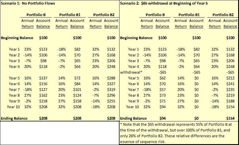
This phenomenon is illustrated by the following example, using the same “Portfolio B” we introduced in our prior example. We have added Portfolio B1, which has the same set of periodic returns as Portfolio B, but they are sequenced differently so that the lowest returns occur first. We also have added Portfolio B2, in which the same periodic returns are sequenced in reverse order compared to Portfolio B1. In Scenario 1, there are no flows into or out of the portfolio. Note that the ending balances for Portfolios B, B1, and B2 are all the same in this scenario. In Scenario 2, we introduce a $65 withdrawal at the beginning of year 5. The difference in ending balances among the three portfolios in this scenario is striking — in fact, Portfolio B1 is wiped out. This highlights the fact that when low or negative returns occur in early periods when withdrawals are being made, they can have a lasting adverse effect and significantly impair the financial well-being of the investor. Scenario 2 dramatically demonstrates sequence risk.
Recent retirees with low non-portfolio income and high early expenses are particularly vulnerable to sequence risk.
There are a few ways to mitigate sequence risk. One is to have no flows — deposits or withdrawals — into or out of the portfolio (as in Scenario 1). However, this is patently unrealistic for most investors. Another way is to successfully avoid making withdrawals for a time after a significant decline in the portfolio’s value. This might be accomplished by keeping a sizeable cash reserve outside the portfolio to cover this contingency. However, the size of the reserve necessary to achieve meaningful immunization against contingencies of unknown frequency and severity may be so large that the long-term “cash drag” on performance may outweigh the benefits, as a number of studies in the financial literature have demonstrated.[1]
The most productive way to control sequence risk is to not have an erratic series of returns — the more stable the return stream, the less the sequence risk. A perfectly smooth return stream, such as that of Portfolio A in first example, has precisely zero sequence risk. (This is a given, since all sequencings of identical periodic returns are indistinguishable from each other.) It does not matter when deposits or withdrawals occur in such a portfolio. While no practical RMI technique can totally eliminate return volatility, every step in that direction adds value from a sequence risk perspective.
The value of stability in mitigating sequence risk should be clear and can be quantified using the approach we have outlined.
There are likely many questions you have about RMI, including those we posed earlier in this series. How can RMI actually provide equity risk management? At what cost? Is the cost so high and/or the upside potential of equities so diminished by RMI that it is not cost-effective over a full market cycle? What would an RMI-infused portfolio look like, and what would its risk/return profile be? We will address these questions in future installments. As always, we encourage your feedback along the way.
Jerry Miccolis is the Founding Principal and Chief Investment Officer at Giralda Advisors, a participant in the ETF Strategist Channel.
This material is for informational purposes only. Nothing in this material is intended to constitute legal, tax, or investment advice. Investing involves risk including potential loss of principal.