Summary­

• Yield curve changes over time can be decomposed into Level, Slope, and Curvature changes, and these changes can be used to construct portfolios.
• Market shocks, monetary policy, and preferences of different segments of investors (e,g. pensions) may create trends within these portfolios that can be exploited with absolute and relative momentum.
• In this commentary, we investigate these two factors in long/short and long/flat implementations and find evidence of success with some structural caveats.
• Despite this, we believe the results have potential applications as either a portable beta overlay or for investors who are simply trying to figure out how to position their duration exposure.
• Translating these quantitative signals into a forecast about yield-curve behavior may allow investors to better position their fixed income portfolios.

It has been well established in fixed income literature that changes to the U.S. Treasury yield curve can be broken down into three primary components: a level shift, a slope change, and a curvature twist.

A level change occurs when rates increase or decrease across the entire curve at once.  A slope change occurs when short-term rates decrease (increase) while long-term rates increase (decrease).  Curvature defines convexity and concavity changes to the yield curve, capturing the bowing that occurs towards the belly of the curve.

Obviously these three components do not capture 100% of changes in the yield curve, but they do capture a significant portion of them. From 1962-2019 they explain 99.5% of the variance in daily yield curve changes.

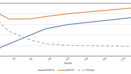
We can even decompose longer-term changes in the yield curve into these three components.  For example, consider how the yield curve has changed in the three years from 6/30/2016 to 6/30/2019.

Source: Federal Reserve of St. Louis.

We can see that there was generally a positive increase across the entire curve (i.e. a positive level shift), the front end of the curve increased more rapidly (i.e. a flattening slope change) and the curve flipped from concave to convex (i.e. an inverted bowing of the curve).

Using the historical yield curve changes, we can mathematically estimate these stylized changes using principal component analysis.  We plot the loadings of the first three components below for this three-year change.

Source: Federal Reserve of St. Louis.  Calculations by Newfound Research.

So why might this be useful information?

First of all, we can interpret our principal components as if they are portfolios.  For example, our first principal component is saying, “buy a portfolio that is long interest rates across the entire curve.”  The second component, on the other hand, is better expressed as, “go short rates on the front end of the curve and go long rates on the back end.”

Therefore, insofar as we believe changes to the yield curve may exhibit absolute or relative momentum, we may be able to exploit this momentum by constructing a portfolio that profits from it.

As a more concrete example, if we believe that the yield curve will generally steepen over the next several years, we might short 2-year U.S. Treasury futures and buy 10-year U.S. Treasury futures.  The biggest wrinkle we need to deal with is the fact that 2-year U.S. Treasury futures will exhibit very different sensitivity to rate changes than 10-year U.S. Treasury futures, and therefore we must take care to duration-adjust our positions.

Why might such changes exhibit trends or relative momentum?

• During periods where arbitrage capital is low, trends may emerge. We might expect this during periods of extreme market shock (e.g. recessions) where we might also see the simultaneous influence of monetary policy.
• Effects from monetary policy may exhibit autocorrelation. If investors exhibit any anchoring to prior beliefs, they might discount future policy changes.
• Segmented market theory suggests that different investors tend to access different parts of the curve (e.g. pensions may prefer the far end of the curve for liability hedging purposes). Information flow may therefore be segmented, or even impacted by structural buyers/sellers, creating autocorrelation in curve dynamics.

In related literature, Fan et al (2019) find that the net hedging or speculative position has strong cross-sectional explanatory power for agricultural and currency futures returns, but not in fixed income markets.  To quote,

“In sharp contrast, we find no evidence of a significant speculative pressure premium in the interest rate and fixed income futures markets. Thus, albeit from the lens of different research questions, our paper reaffirms Bessembinder (1992) and Moskowitz et al. (2012) in establishing that fixed income futures markets behave differently from other futures markets as regards the information content of the net positions of hedgers or speculators.  A hedgers-to-speculators risk transfer in fixed income futures markets would be obscured if agents choose to hedge their interest rate risk with other strategies (i.e. immunization, temporary change in modified duration).”

Interestingly, Markowitz et al. (2012) suggest that speculators may be profiting from time-series momentum at the expense of hedgers, suggesting that they earn a premium for providing liquidity.  Such does not appear to be the case for fixed income futures, however.

As far as we are aware, it has not yet been tested in the literature whether the net speculator versus hedger position has been tested for yield curve trades, and it may be possible that a risk transfer does not exist at the individual maturity basis, but rather exists for speculators willing to bear level, slope, or curvature risk.

Click here to read the full article on Newfound Research’s website.