By Corey Hoffstein, Newfound Research
A few months ago, in our presentation All About Factors & Smart Beta[1], we introduced the basics of factor investing. The core concept is that securities are ranked based upon a scoring system, and a self-financing portfolio is built by short-selling poorly ranking securities and using the proceeds to buy high ranking securities.
The self-financing nature of the portfolios – also called “dollar neutral” portfolios – makes factor performance easy to calculate. It does, however, introduce an interesting quirk: the portfolios are not beta neutral.
In other words, if we look at our long/short factor portfolio as two separate legs – a long leg and a short leg – the sensitivity each leg has to overall market moves can be very different. Furthermore, the sensitivity of each leg can evolve over time. This means that the overall factor portfolio can not only end up with sensitivity to market moves, but time-varying sensitivity.
Consider, for example, the value factor. Below we plot the beta of the long leg minus the beta of the short leg.
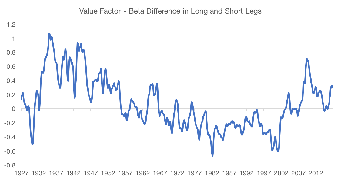
Source: Kenneth French Data Library. Calculations by Newfound Research.
Not only do we see that the magnitude of the beta difference can be quite large, we see that it can vary drastically over time. In addition to a broad swing from +1 to -0.7 from the 1930s to the 1980s, there are many dramatic short-term swings as well.
This raises two interesting questions:
- Are factor returns a byproduct of non-zero beta exposure?
- Do factors benefit from time-varying beta exposure – i.e. “market timing”?
Data & Methodology
Data in this commentary comes from the Kenneth French data library. For value and size factors, we utilize the “Hi 30” and “Lo 30” portfolios provided. For the momentum factor, we equally-weight the top and bottom three deciles to create synthetic “Hi 30” and “Lo 30” portfolios.
To estimate betas, we run rolling 25-week regressions of Hi and Lo portfolio excess returns against market excess returns. We then apply a 12-week exponentially weighted smoothing process to help eliminate noise.
First, an important tangent…
It is worth pointing out that this is the wrong way to do this. To actually estimate the beta of each leg, we should first find the beta of each underlying stock and then calculating the weighted average across all stocks in the portfolio. Without access to the underlying components, however, we are using past realized returns as a proxy estimate for present value. This is likely okay for low turnover factors like value and size, but may make the estimate for a higher turnover factor like momentum less accurate.
Furthermore, beta is merely a statistical tool we use to conveniently summarize a relationship; it is not an intrinsic property of a company. So we are estimating something that, in and of itself, is an estimate based on past behavior. Even if our estimate is completely certain, the model may be completely wrong. Hence, this entire analysis may just be a big case of garbage in, garbage out. You’ve been warned!
Okay, back to the regularly scheduled programming.
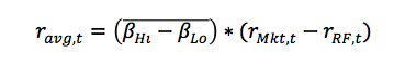
To test whether factors benefit from long-term beta exposure, we’ll create a portfolio whose monthly excess return is: