
By Nathan Faber, Newfound Research
Diversification is a common topic in portfolio construction. Rather than serving as the sole, quantifiable objective, it is most often either pursued in tandem with another objective – such as return maximization – or pursued simply by including more asset classes or adding constraints based on intuition (e.g. position size limits).
But it does not have to be this way; diversification can be pursued explicitly as the sole objective in portfolio construction.
In the 2008 paper, Toward Maximum Diversification, the diversification ratio, D, of a portfolio, w, is defined as:
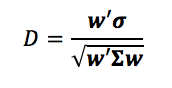
where σ is the vector of volatilities and Σ is the covariance matrix. The term in the denominator is the volatility of the portfolio and the term in the numerator is the weighted average volatility of the assets. More diversification within a portfolio decreases the denominator and leads to a higher diversification ratio.
The authors propose maximizing this ratio as a portfolio construction technique.
Like all portfolio construction methods, there are a set of assumptions that have a bearing on the results and conditions under which this portfolio will be optimal, and it is beneficial to examine both of these before blindly seeking diversification for diversification’s sake.
Assumptions Behind Maximizing Diversification
According to the portfolio construction flow chart in ReSolve Asset Management’s article titled Portfolio Optimization: A General Framework for Portfolio Choice, constructing the maximum diversification portfolio means that we have active views on volatilities and correlations, confidence in our ability to estimate them, no active views on returns, the belief that markets are risk-efficient, and that markets reward total risk.
Whether we explicitly acknowledge these assumptions is irrelevant. They are made nonetheless.
Using a cross-section of asset classes going back to 1973, we can construct long-only portfolios that maximize the diversification ratio using a 3-year rolling covariance matrix.
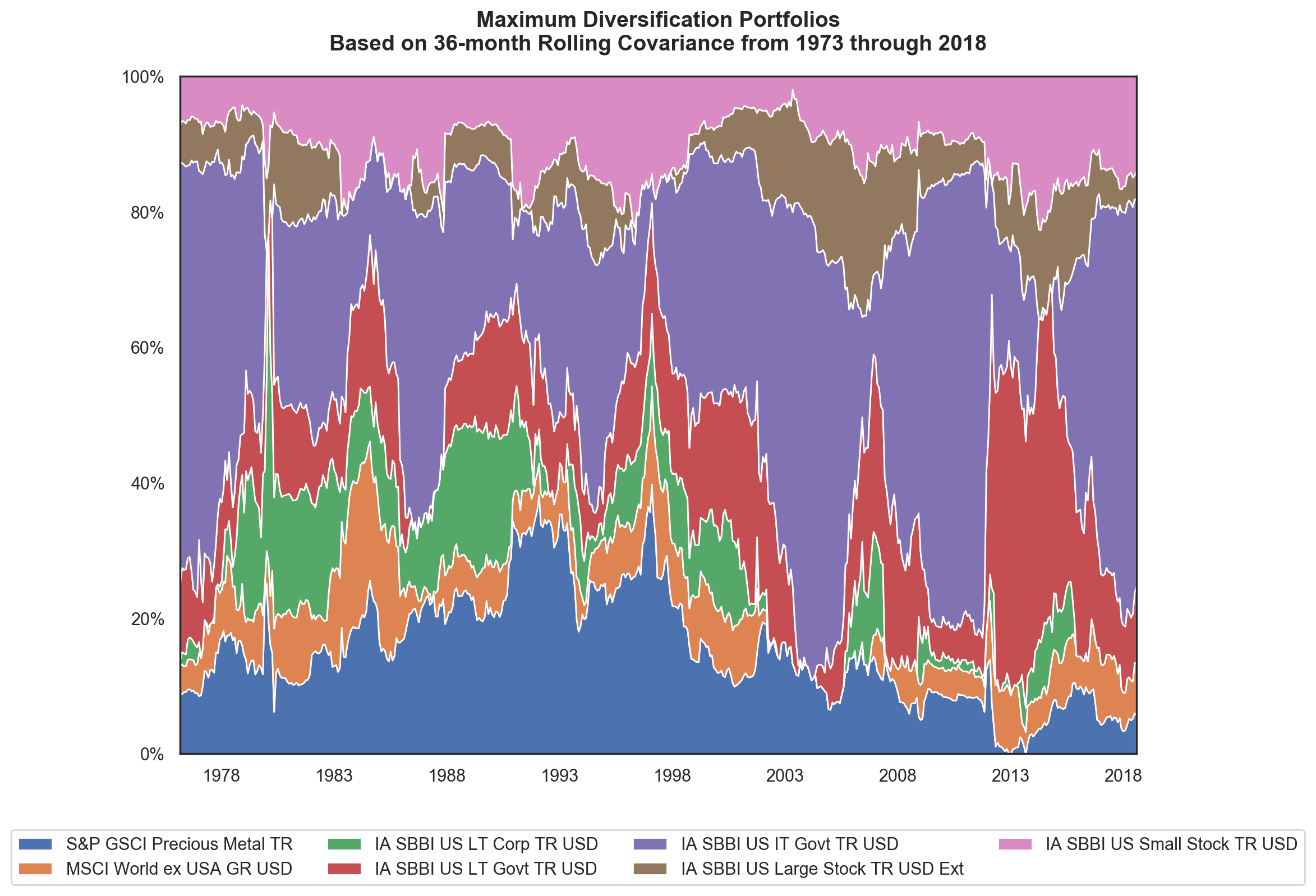
Over time we see some significant shifts in the allocation to precious metals, peaking around 40% and declining to 0%. The overall bond allocation ranges between 30% and 75% with an average of about 60%, and equities range from 15% to 40% with an average around 25%. The concentration seen in certain asset classes and the large swings in allocations demonstrate that the mathematical measure of diversification employed herein may not always align with a more intuitive expression of the concept.
We can also see that the bond split across the term and credit spectrum and the equity split across size and geographies varies as diversification benefits ebb and flow within the asset classes.
The diversification ratio of these portfolios also varies considerably over time as correlations and volatilities fluctuate. Over some periods, it appears that the portfolio has a significant amount of internal diversification with a ratio approaching 3. At other times, the ratio is closer to 1.5, meaning that the expected volatility of the portfolio is only 33% less than if all the assets were perfectly correlated.
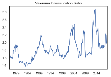
Static asset allocations can vary substantially in their diversification benefit as the markets evolve, and this graph highlights how much diversification changes even if we are flexible with the allocations we choose.
These diversification ratios are what we expected based on the trailing covariance data: but diversification can come and go from one period to another. The realized diversification ratio can be very different (green line in the following chart) and will be bounded by the maximum diversification ratio (orange line) over the out-of-sample period; that is, the diversification achievable if we had perfect foresight. This realized and potential diversification can be very different from the ex-ante diversification ratio (blue line) used in portfolio construction.
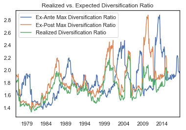
In the recent months, the maximum expected diversification ratio has been around 2. The confidence in the covariance matrix estimate will determine how close this is to reality going forward.
Optimal Diversification
From the perspective of Sharpe ratio maximization, the maximum diversification portfolio is only going to be optimal ex-post if the realized excess returns are proportional to the volatilities. This implies constant Sharpe ratios for all assets through time.
