
By Corey Hoffstein, Newfound Research
There are articles that, after we read them, we say, “we wish we had written that.” Recently, our friends over at ReSolve Asset Management published one such article titled Portfolio Optimization: A General Framework for Portfolio Choice, wherein they rebuild the theoretical foundation behind different optimization techniques based upon implied assumptions and beliefs.
The whole paper is worth a read, but the following decision tree should really be taped above the computers of anyone constructing portfolios.
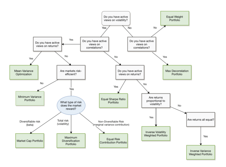
Source: ReSolve Asset Management. Reprinted with permission.
What makes this diagram so powerful, in our opinion, is that it connects different portfolio schemes together based upon our beliefs, both in what we know and how confident we are.
The choice of employing a maximum diversification portfolio, for example, is not just an expression of our desire to increase diversification within our portfolio. The choice necessarily implies that we have active views on both risk and correlations and believe that the market compensates investors for total risk borne. If we do not actually hold these views, then choosing maximum diversification for our portfolio construction technique may be sub-optimal.
(The notion of approaching portfolio construction from “first principles” is a topic we discussed with ReSolve’s Chief Investment Officer, Adam Butler, on our podcast; listen here and here.).
When it comes to portfolio construction, however, having a belief is one thing. One’s confidence in that belief is another. For example, I may believe in the momentum anomaly and therefore hold active views on future returns based upon recent realized returns. How confident I am in those views will ultimately dictate how and to what extent the views influence my portfolio construction. If I can go one step further and actually quantity my confidence, then I can attempt to directly account for it.
These are implementation topics we have discussed in the past (see our commentary Combining Tactical Views with Black-Litterman and Entropy Pooling), but we wanted to explore how implementation decisions in portfolio construction (so-called “craftsmanship”) can have an outsized impact over the short-term.
Measure Twice, Transform Once
By way of example, we will construct a sector rotation portfolio. Specifically, every day we will measure the 12-1 month total return for each of the primary equity sectors as well as estimate their covariance using exponentially-weighted daily returns. With this data in hand, we will calculate the Sharpe-optimal portfolio.
Let’s pause for a moment and consider the implications of our decisions.
- We hold active views on volatility, correlations, and returns;
- We believe we can quantify these views; and
- We are 100% confident in our estimates.
While the diagram above is a guide for (1), it does not outright address (2) or (3). Consider, for example, if we held active views on volatility, correlations, and returns, but had zero confidence in our return forecasts (say because we picked them out of thin air). While the mean-variance optimization would still be the theoretically correct choice for what we believe, it is pragmatically incorrect; we would be better off saying we have no view on returns.
The trouble lies in the middle zone: where we have less than 100% confidence in our estimates. Which is usually the case as our estimates are exactly that: estimates. The precision of a dozen decimal places belies the fact that the figures are actually shrouded in a probability distribution.
What if, for example, we believed that our estimates for returns were accurate relative to one another (i.e. ordinally correct) but incorrect in their precision. In other words, we’re generally confident that the rank order of returns will be preserved, but not very confident in the dispersion between returns (e.g. we believe that Apple will outperform Google but have no idea if Apple will return 5% and Google 4% or if Apple will return 5% and Google -50%)?
One potential solution might be to “transform” the data.
Transformations are merely functions applied to the data that help isolate a particular feature or characteristic. With respect to the expected return data in question here, there are two important features: level and dispersion. Level tells us the average return, while dispersion tells us how close or far the data points are from that average.
It should be noted that in mean-variance optimization, the result is invariant to the scale of the data. In other words, we can multiply our expected returns by any constant and the resulting optimal portfolio will not change. This is important in terms of thinking about the transformations below, as information about level is only eliminated in the case where the data is explicitly de-meaned.
For example, calculating the cross-sectional z-score of expected returns will explicitly de-mean the data. However, the second step – dividing by the standard deviation of the data – merely scales the information, which has no effect. Therefore, z-scoring eliminates level information, but preserves dispersion information. Rank ordering our data, on the other hand, preserves level information (since we can simply scale the data to have a new mean) but eliminates some, though not all, information about the dispersion.
Below we list several potential transforms, as well as general thoughts about how they affect level and dispersion. By no means is it a complete list.
The Identity Transform
This transform simply multiplies the data by one, preserving all information.
Z-Score Transform
This transform calculates a cross-sectional z-score across the data. By first subtracting the mean of the data, all level information is eliminated. All dispersion information, however, is retained.
The effect of this transformation, in the case of mean-variance optimization, is that assets with returns below the mean will now only be included in the portfolio if they have beneficial diversification properties. As example, consider an optimization over five asset classes with the following expected returns:
- Asset A: 20.0%, Asset B: 19.0%, Asset C: 18.0%, Asset D: 17.0%, Asset E: 16.0%
- Asset A: 12.6%, Asset B: 6.3%, Asset C: 0.0%, Asset D: -6.3%, Asset E: 12.6%
If we z-score this data, and assuming the same covariance structure, then our optimized portfolio would have the same allocations.
Logistic Transform
The logistic transform retains information about level but reduces information about dispersion.
The growth rate of the logistic function plays an important role in the amount of dispersion information retained. In fact, in many ways, a logistic transform can be thought of as a more generalized function for transforms discussed below. When the growth rate is zero, all dispersion information is eliminated. When growth rates are small, the transform approaches a rank transformation (discussed below) except in the extreme trails. High growth rates cause the logistic function to approach a step function (discussed below).
For middle-ground growth rates, relative scale of outliers is compressed while the scale between data around the mean is made more uniform.
