
A Case Study on Currency Hedging Emerging Market Equities
When it comes to investing, risk management is of utmost importance. But, beyond simply measuring investment risk, as you may know, investors also aim to contextualize portfolio return by the risk taken on to achieve that return. This blog focuses on this concept and then puts it to work in a case study on currency hedging a broad market-capitalization weighted emerging markets equity index.
Let’s begin by defining a common metric that investors use to gauge investment risk: standard deviation. By its definition, standard deviation measures the level of dispersion that a dataset has around its mean. In finance, standard deviation gives investors a sense of the historical volatility of investment returns, and it is therefore commonly used to quantify an investment’s level of risk (note that standard deviation assumes that investment returns are normally distributed—which is typically not the case in reality—so it typically serves as a rough approximation of historical investment risk).
But, standard deviation on its own is not entirely useful. Yes, it explains how volatile an investment may have been in the past, but it does not consider that investment’s level of return. Suppose that a higher volatility (i.e. more risky) investment provided investors with higher return than a lower volatility (i.e. less risky) investment. At first glance, one may conclude that the higher risk investment is better than the lower risk investment—after all turning $100 into $110 potentially sounds more attractive than turning $100 into $105 over the same time period. However, the answer to whether the higher-return investment is truly the more attractive option depends on how much risk was taken on to achieve the return. In other words, what if the investment that had a 5% return is one tenth as risky as the investment that had a 10% return? This is where the concept of the Sharpe Ratio comes in. Named after Nobel laureate William Sharpe, the Sharpe ratio compares investments on a risk-adjusted basis. It is calculated by taking the return of an investment over a period and subtracting a risk-free rate of return over that period (the return on a US Treasury serves as a proxy for the risk-free rate) and then dividing the entire quantity by the investment’s volatility (standard deviation) over the period.
Let’s take a look at what the Sharpe ratio tells us about the investments in the aforementioned example. Suppose that the first investment that returned 10% (i.e. turned 100 into 110) had a volatility (standard deviation) of 10%. Then suppose that the second investment that returned 5% (i.e. turned 100 into 105) had one tenth that level of volatility, or 1%. Assuming that the risk free rate is zero, the Sharpe ratio for the first, higher-return investment is 1 (calculation: (10% – 0%) / 10% = 1), while the Sharpe ratio for the second, lower-return investment is 5 (calculation: (5% – 0%) / 1% = 5). As you can see, from a risk-adjusted perspective, the investment that returned 5% is significantly more attractive than the investment that returned 10%. In fact, as the Sharpe ratio suggests, it is 5 times more attractive because it earned 5% return per 1% of risk while the other investment only earned 1% return per 1% of risk. Accordingly, investors are more likely to prefer investments that have higher Sharpe ratios over those that have lower Sharpe ratios.
But, how does a portfolio improve upon its Sharpe ratio? Mathematically, and assuming a constant risk-free rate of zero, there are several possible ways to do so: 1) Increasing return without changing risk 2) lowering risk without changing return 3) increasing return by a higher percentage than risk increases 4) decreasing return by a lower percentage than risk decreases. As you may have guessed, achieving these outcomes is no easy feat. As I allude to in a prior blog (see Why investing overseas may be better than you think), diversifying a portfolio is one of the simplest ways to improve its Sharpe ratio. (Of course, diversification does not ensure a profit or protect against a loss.) But, other thoughtful investment strategies can also improve a portfolio’s Sharpe ratio. The following case study takes a look at how investing in emerging market equities on a currency hedged basis, forms an interesting narrative when it comes to improving a portfolio’s Sharpe ratio.
Case Study: Currency Hedging a Broad Market-Capitalization Weighted Emerging Markets Equity Exposure
This case study compares the MSCI Emerging Markets Unhedged Index to the MSCI Emerging Markets Currency-Hedged Index to demonstrare how hedging currency risk in a portfolio of market-capitalization weighted emerging markets equities would have impacted that portfolio’s Sharpe ratio over time.
To begin, Exhibit 1 shows the difference in rolling 1-year volatility between the MSCI Emerging Markets Unhedged Index and the MSCI Emerging Markets Currency-Hedged Index from 12/18/2002 to 5/9/2019. (This period was chosen due to a lack of data availability prior to 12/18/2002).
Exhibit 1:
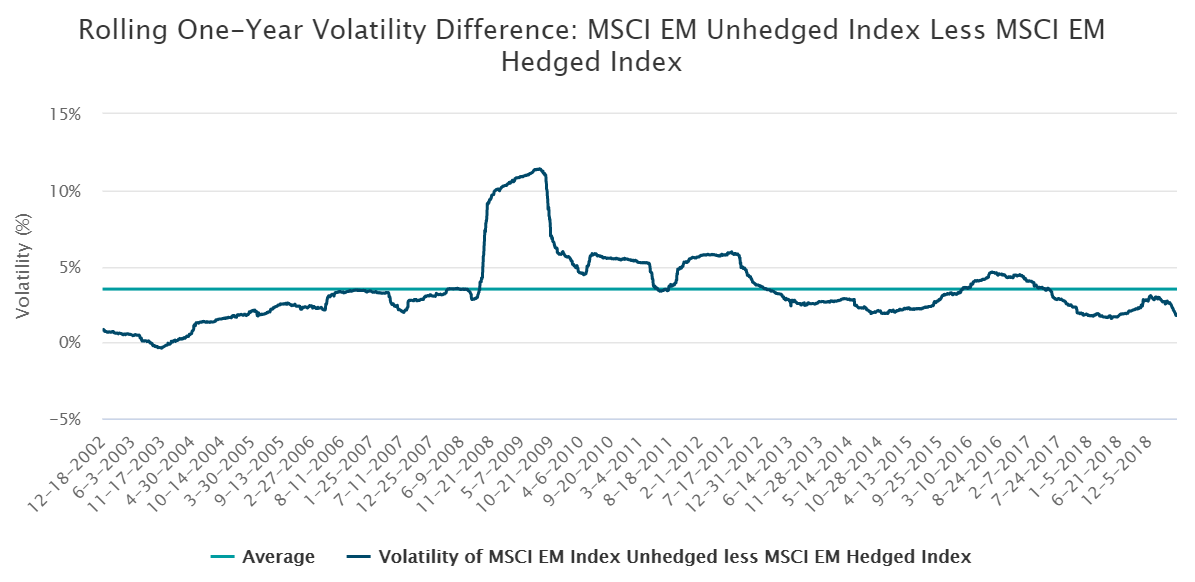
Source: Bloomberg and DWS as of May 10, 2019. Performance is historical and does not guarantee future results. Index returns assume reinvestment of all distributions and do not reflect fees or expenses. It is not possible to invest directly in an index. 1-year rolling volatility was calculated using daily return data. This graph is for illustrative purposes only.
As you can see, hedging currencies significantly reduced risk (by an average of about 3.5% across the period shown). But, as mentioned above, risk is only one part of a holistic view of a portfolio. The next step involves examining risk-adjusted returns by looking at the portfolio’s Sharpe ratio over time, shown in Exhibit 2.
Exhibit 2:

Source: Bloomberg and DWS as of May 10, 2019. Performance is historical and does not guarantee future results. Index returns assume reinvestment of all distributions and do not reflect fees or expenses. It is not possible to invest directly in an index. Sharpe Ratios were calculated using monthly return data. The Bloomberg Barclays US Treasury Bills: 1-3 Month Total Return Index served as a proxy for the risk free rate. The currency hedged index is the MSCI Emerging Markets 100% Hedged Net Total Return USD Index, while the unhedged index is the MSCI Emerging Markets Net Total Return USD Index. This graph is for illustrative purposes only.
The shaded areas show time frames over which hedging currency risk from a portfolio of emerging market equities improved that portfolio’s Sharpe ratio relative to a portfolio that did not hedge currency risk. As you can see, after mid-2007, more often than not hedging currency risk improved the Sharpe ratio. But why is this? To get a better sense of what drove the improved Sharpe ratio, we deconstruct the ratio into its two components, a numerator (i.e. return minus the risk-free rate) and a denominator (i.e. standard deviation). Exhibit 3 shows the numerator (i.e. rolling 36 month return minus the risk-free rate for the MSCI emerging markets hedged and unhedged indexes), and Exhibit 4 shows the denominator (i.e. rolling 36 month standard deviations for both indexes).
Exhibit 3:
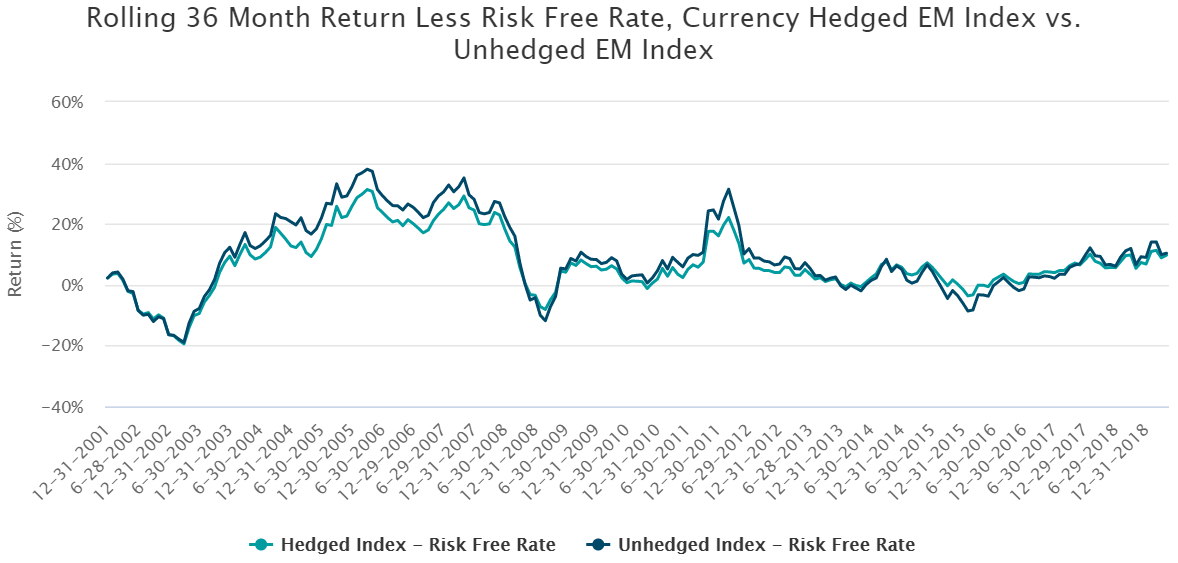
Source: Bloomberg and DWS as of May 10, 2019. Performance is historical and does not guarantee future results. Index returns assume reinvestment of all distributions and do not reflect fees or expenses. It is not possible to invest directly in an index. The Bloomberg Barclays US Treasury Bills: 1-3 Month Total Return Index served as a proxy for the risk free rate. The currency hedged index is the MSCI Emerging Markets 100% Hedged Net Total Return USD Index, while the unhedged index is the MSCI Emerging Markets Net Total Return USD Index. This graph is for illustrative purposes only.
From a return perspective, Exhibit 3 shows that there are only slight differences between the hedged and unhedged versions of the MSCI emerging markets index, but not much in the way of an obvious strong relationship or trend. (Note: it is important to keep in mind that hedging emerging market currencies has typically cost US investors a cost of carry since emerging markets interest rates have been higher than interest rates in the US. The opposite has been true when currency hedging developed markets: US investors have been paid a cost of carry since developed market interest rates have been lower than interest rates in the US. For simplicity, this blog does not focus on these costs of carry). However, from a volatility perspective, Exhibit 4 shows that there was a pronounced difference between the hedged and unhedged indexes.
Exhibit 4:

Source: Bloomberg and DWS as of May 10, 2019. Performance is historical and does not guarantee future results. Index returns assume reinvestment of all distributions and do not reflect fees or expenses. It is not possible to invest directly in an index. The currency hedged index is the MSCI Emerging Markets 100% Hedged Net Total Return USD Index, while the unhedged index is the MSCI Emerging Markets Net Total Return USD Index. This graph is for illustrative purposes only.
Across the entire period observed (2001 to 2019), the unhedged index had systematically higher volatility than the hedged index. We attribute this higher level of volatility to the currency exposure, and the chart shows that the difference in volatility became more pronounced in later years (i.e. in the period after the financial crisis of 2007-2008 to present day) which roughly corresponds with the time period in Exhibit 2 that showed higher Sharpe ratios for the currency hedged index relative to the unhedged index more often than not. The reason that volatility of the unhedged index rose after the financial crisis potentially had to do with the level of correlation between emerging market currencies and their corresponding local equity markets over time, shown in the next exhibit.
Exhibit 5:

Source: Bloomberg and DWS as of May 10, 2019. Note that investors cannot invest directly in an index. This graph is for illustrative purposes only.
Visually, it appears that there were roughly two correlation regimes, before and after the financial crisis of 2007-2008. Compared to pre-crisis correlations, higher correlations post-crisis meant that hedging currency risk became an even more useful risk reduction tool and Sharpe ratio improver (as evidenced in Exhibit 2). This result makes sense because, as correlations between assets in a portfolio rise, the benefits to diversification within that portfolio tend to diminish and portfolio risk increases. In this case, unhedged emerging market equities can be considered a two asset portfolio consisting of the MSCI Emerging Market Equity Index and the associated MSCI Emerging Market Currencies Index.
In conclusion, we hope that this blog provides investors with a better understanding of the importance of analyzing risk-adjusted returns. The case study shows that though there is no investment strategy that can guarantee consistent Sharpe ratio improvement, investors can gain deep insight into when and why a strategy works to improve risk-adjusted returns. In the case of emerging markets, though currency fluctuations consistently added volatility to a portfolio of unhedged emerging market equities, only after correlations between the performance of emerging market equity markets and their currencies rose, post-crisis, did hedging that currency risk prove most beneficial. For investors interested in considering currency hedging international equities, there are a wide range of currency hedged equity ETFs available in the market today. For additional information on currency hedging, read white paper on currency hedging.