
Deep neural network models are growing rapidly to improve accuracy in many different applications, e.g. language modeling, machine translation, and speech and image recognition.
As the models grow, the compute and memory resources to train those models also increase proportionally. Since the growth of compute and memory resources are not as fast as the models, researchers are coming with many techniques to train the models faster, e.g. reduced precision representation, sparse models, and compressed models. In this blog post, we evaluate the scope of mixed precision numbers in training deep neural networks for end-to-end application (e.g. language modeling). We show that training with mixed precision allows us to achieve 4.1X performance improvement compared to single precision floating point numbers.
Deep learning models are usually trained using 32-bit single precision numbers (FP32). In this work, we use the technique for mixed precision discussed in [1], where we use 16-bit floating point numbers (FP16) to (i) reduce the memory needed to train the deep learning models and (ii) take advantage of faster computational units for FP16 (e.g. TensorCore in NVIDIA’s V100 processor). We use FP16 for the inputs, weights, activations and gradients of the models. However, due to the limited mantissa in FP16 compared to FP32, we maintain a master copy of the weights in FP32. This FP32 master copy is rounded to FP16 only once for the forward and backward propagation to perform FP16 arithmetic computation on the faster hardware. To minimize gradient values becoming zeros, we use loss scaling (multiplying the loss by a scaling factor, S, e.g. 256 and 512 before computing gradients and then dividing the gradients by S before applying to the weights). Since we use both FP16 and FP32 in our approach, we denote this method as mixed precision technique (MP), similar to [1]. More details on these are available at [1, 2, 3].
![]()
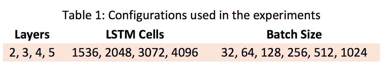
We use the word language models (WLM) for the experiments. The stack of recurrent layers in WLMs are shared by many different applications like speech recognition and machine translation. We vary the three parameters in the experiments, the number of recurrent layers, the batch size used for training, and the number of cells in each recurrent layer, denoted by L, B, and N respectively. Table 1 shows the detail configurations. We use Basic LSTM cells [5] for each recurrent layer and use SGD optimizer with momentum along with learning rate decay and dropout [4]. We profile all the word language models using the Penn Tree Bank (PTB) dataset [3]. We perform FP16 arithmetic using DGX system of NVIDIA, which consists of 8 Tesla V100 GPUs. We use a single V100 GPU with CUDA 9.1.85 and CUDNN 7.0.5 for the experiments. The kernel execution times are measured by NVIDIA’s CUPTI library 10.0.
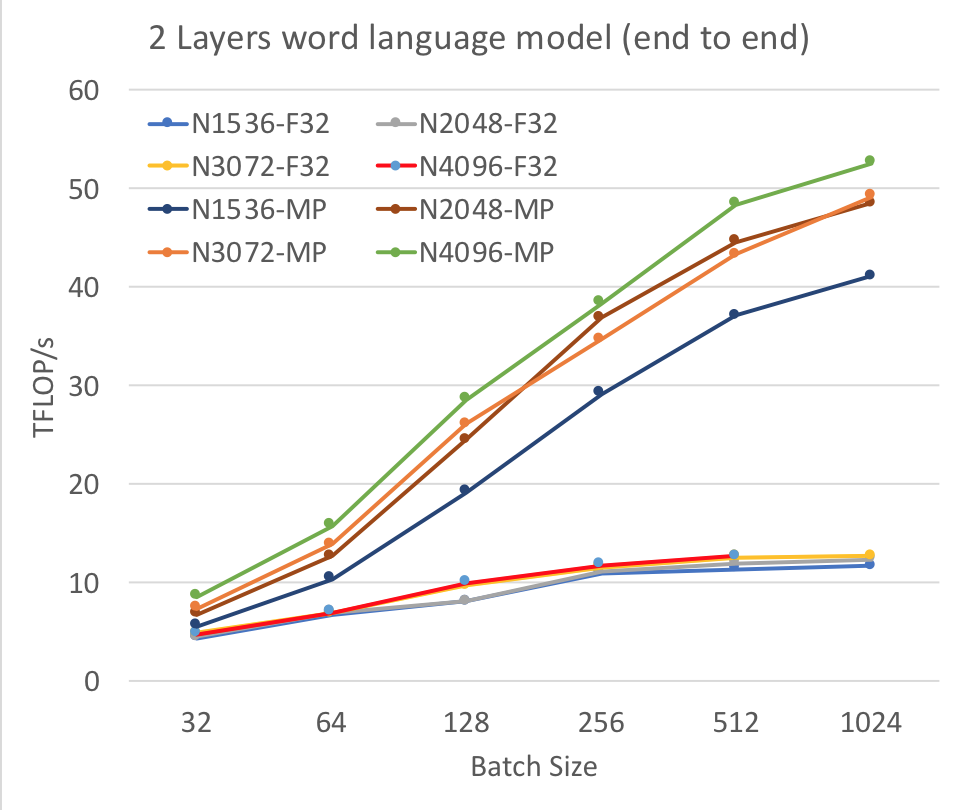
Figure 1: End-to-end achieved FLOP per second for word language model using 2 LSTM layers. N1536 denotes that the number of LSTM cells per layer is 1536.
We now present the results of our experiments. We first demonstrate how end-to-end Floating-Point Operations per second (FLOP/s) changes as we vary the batch size and the LSTM cell size. We vary these as per Table 1 keeping the layer size, L constant (L=2). As shown in Figure 1, when we increase the batch size, the achieved FLOP/s increases at a higher rate for mixed precision (MP) than single precision, FP32. At batch size 256, FP32 saturates, whereas MP keeps increasing, but the rate slows down after batch size of 512. As the size of the LSTM layers gets bigger, the achieved FLOP/s also increase. We achieve a maximum of 52.6 TFLOP/s using mixed precision, 4.1X performance improvement compared to achieved 12.7 TFLOP/s using FP32. We observe that the system runs out of memory for FP32 when the batch size is 1024 and the number of LSTM cell is 4096. In contrast, the model runs smoothly for the same configuration using mixed precision, primarily due to the reduced memory requirement (almost half). We achieved similar end-to-end performance gain when we varied the number of layers to 3-5. It is worthwhile to mention that we observe the achieved peak utilization by mixed precision (42%) is much lower than FP32 (81%) on Tesla V100 GPU.
![]()
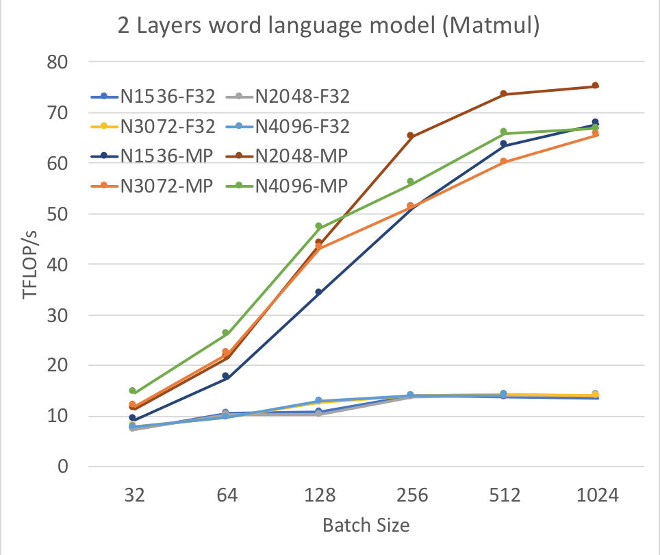
Figure 2: Achieved FLOP per second by matrix multiplication operation using 2 LSTM layers.