

By Corey Hoffstein, Newfound Research
We like to think that, as quants, our beliefs are ultimately swayed by the weight of the evidence. But there are a few artifacts that arise from the data that are, quite simply, just hard for us to get behind.
Seasonality is one of those effects.
Candidly, we had not given seasonality the time of day until recently. Earlier this year, I had the pleasure of speaking at the Democratize Quant conference, hosted by our friends at Alpha Architect. My presentation was on the effects of timing luck, an idea that quite simply says, “when you form your portfolio can have a significant impact on your results.” Our research has largely been around the randomness of this impact, with the assumption that when is not a source of edge, but rather a source of noise that should be diversified away.
After presenting, Alpha Architect’s co-CIO’s Wes Gray and Jack Vogel shared with me some of the literature on seasonality, which argue that when may actually be a significant source of edge. Many of these papers highlighted the more well-established anomalies – like the turn-of-month, turn-of-quarter, and January effects – which many argue are tied to investor behavior (window dressing and tax-loss harvesting).
These are not insignificant effects. Consider the following image and table from the recently published Fact, Fiction, and the Size Effect by Alquist, Israel, and Moskowitz (2018).
![]()

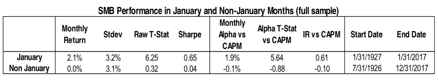
We can see that the size effect is subject to a large seasonality effect. In fact, the entire premium comes from the month of January.
Another popular anomaly is the Halloween indicator, commonly known by the rhyme scheme “sell in May and go away.” Jacobsen and Zhang (2014) fail to reject the existence of the anomaly in 65 different countries and replicate a 2002 study to demonstrate that in the 37 countries studied, the effect remains present out-of-sample. Despite significant effort to explain the effect, no critique survives analysis other than the fact that everybody is on vacation.
Perhaps the most curious effect, however, is from a paper by Keloharju, Linnainmaa, and Nyberg (2015), in which they find that a strategy which selects stocks based upon their historical same-calendar-month returns earns a significant excess premium.
As an example, at the beginning of January, the strategy would look at the current universe of stocks and compare how they performed, on average, in prior Januaries. The strategy would then buy those stocks that had performed well and short-sell those that had performed poorly.
They also document similar seasonality effects in anomalies (e.g. accruals, equity issuances, et cetera), commodities, and international stock market indices. Further, seasonality effects found in different assets are weakly correlated with one another, indicating the potential to diversify across seasonality strategies that employ the same process.
Indeed, this anomaly proves to be economically significant, incredibly robust, and rather pervasive. So we’ll call it the anomaly that broke the camel’s back, because it has convinced us that seasonality warrants further investigation.
But does it work for sectors?
In this commentary, we will explore whether the anomaly discovered by KLN (2015) proves successful in the context of U.S. sectors. Using data from the Kenneth French data library, we explore three approaches.
- Expanding Window: Select sectors each month based upon full set of prior available data.
- Rolling Window: Select sectors each month based upon the prior 30 years of data.
- EWM: Select sectors each month based upon the full set of prior available data, but weight the influence of the data exponentially (with a center-of-mass at 15 years).
We employ three approaches in effort to determine (1) if the effect is robust to specification, and (2) the stability of the sector recommendations over time.
At the beginning of each month, we construct a long/short portfolio that goes long the three sectors with the highest historical average during that month and short the three sectors with the lowest historical average during that month.
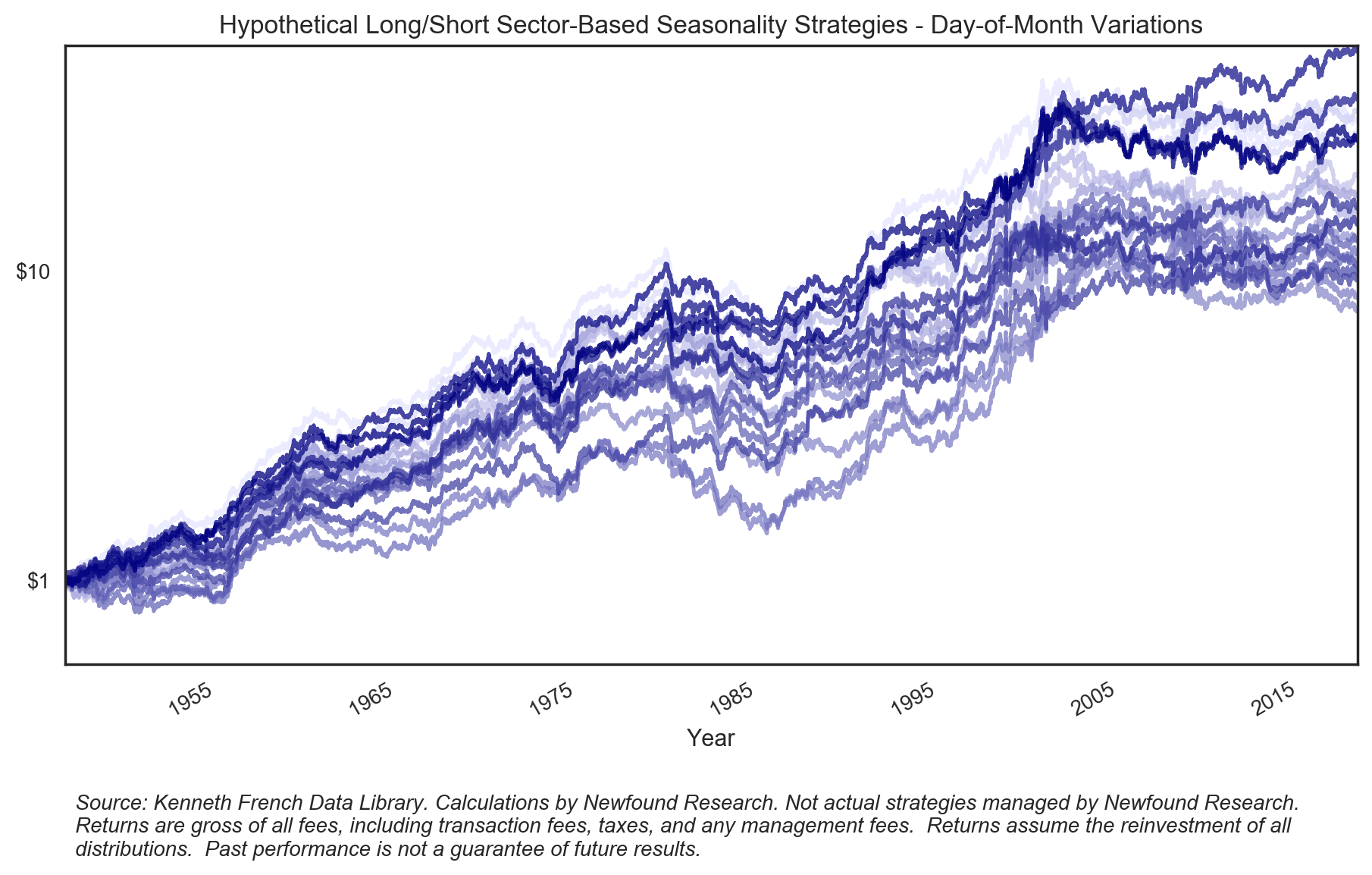
We employ an overlapping portfolio implementation that allows us to account for the potentially arbitrary nature of month definitions. While the traditional Gregorian calendar is one way of dividing the year into 12 months, there is no reason we could not arbitrarily shift the definition forward or backward several days. For example, instead of defining a month using the traditional calendar approach, we could define a month as the 4th to the 4th, or the 21st to the 21st.
By normalizing each month to assume 21 trading days, we can use this approach to create 21 variations of the strategy and determine whether this effect is truly calendar based effect or whether there is a more nuanced seasonality. For instance, there could be an effect that hinges on the period from April 15th to May 15th because of tax day.
Below we plot the 21 variations for the rolling window implementation. While we can see significant variation between the different definitions, all appear to be economically significant over the long-run.
The overlapping portfolios’ implementation can be thought of as, quite simply, the average result of the above variations. We create an overlapping portfolio implementation for each of the three variations and plot the results below.

We can see that while all three variations appear to be economically significant (e.g. the rolling variation generates an annualized return of 4.4% with an annualized volatility of 8.4%), both the rolling and exponentially-weighted approaches significantly outperform the expanding window approach post-1995, indicating that the sectors selected in a given month may not be stable over time.
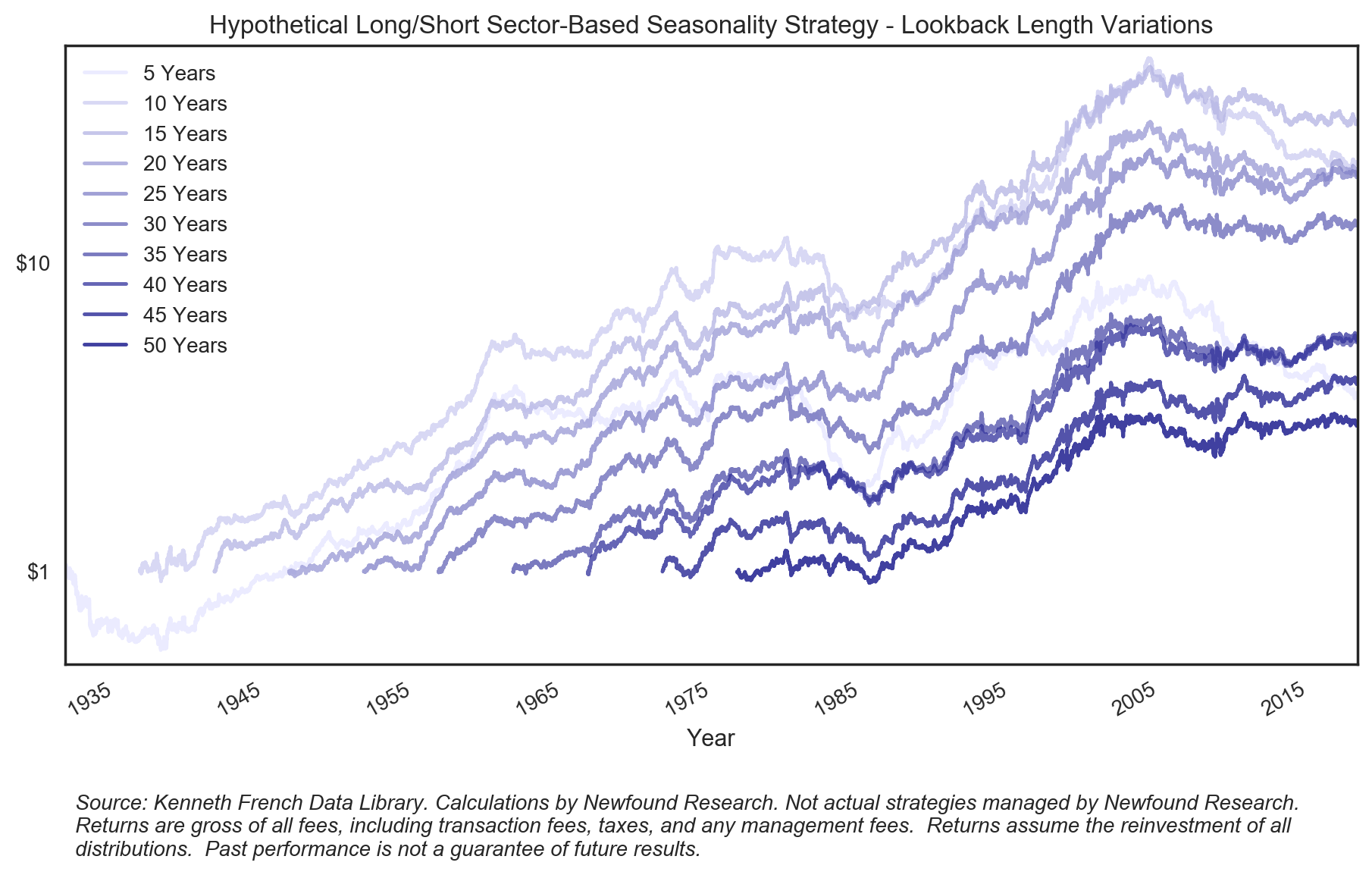
Our choice of using a 30-year lookback window is somewhat arbitrary, informed only by prior literature and an attempt to have a meaningful number of observations for deriving rankings. That said, there is no reason we could not explore the stability of this seasonality effect and its sensitivity to perturbations in the lookback parameter. Below we plot the rolling variation using a range of lookbacks from 5-to-50 years.
We can see that all seem to offer an economically large edge. Due to the fact that the available history for each lookback differs, we can only compare performance across their shared history. In this case, the 25-year lookback maximizes both annualized return and Sharpe ratio over the period. The decline in both return and Sharpe are not purely monotonic as the lookback period increases and decreases, but the 25-year horizon does appear to be a fairly stable maximum.
Recommendation changes over time
To explore the stability of sector selection over time, we look at the identified ranks of each sector for the rolling window implementation in both 1947 and 2017.