

We can see that in several cases, the ranks have taken a complete turn. For example, while in 1947 the Energy sector would have been a short in July, in 2017 it is a long. Similarly, in 1947 Energy was a long in September and October, while in 2017 it was a short. We see similar changes for Durables and Utilities in July and August and Health Care in May and June.
![]()
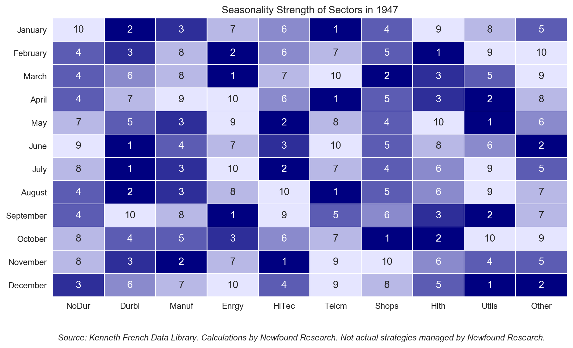
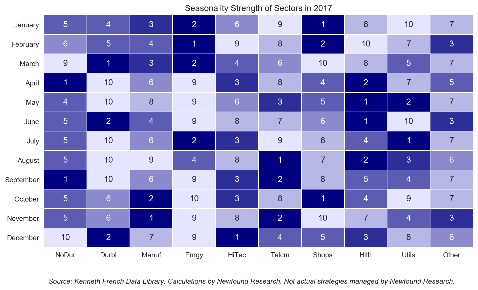
One hypothesis as to why the ranks are not stable is that the composition of the sectors has changed dramatically over time. Consider, for example, that a technology company in 1947 would be meaningfully different than a technology company in 2017. In many ways, these sector definitions are somewhat arbitrary (what is Amazon classified as, again?). Therefore, as new sectors develop over time and compositions change, we might not expect seasonality-based rank order to remain consistent.
Is it significant?
We can begin our analysis of significance by first exploring the different quintile rankings of the strategy (all analysis henceforth is performed using the 30-year rolling window implementation variation).
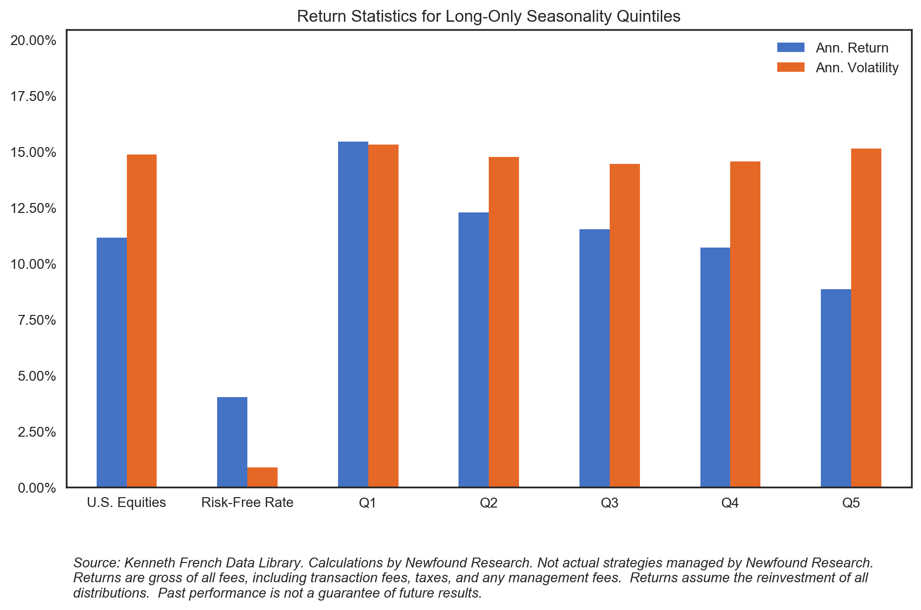
The purpose is two-fold. First, we want to determine how the quintiles do relative to each other. Ideally, we would see a monotonic decrease in annualized performance and a monotonic increase in Sharpe ratio. We do not plot the Sharpe ratio above, but we can see the stead decrease in return with a fairly consistent volatility profile, indicating a decreasing Sharpe ratio as well.
Second, we want to determine how much “alpha” is available for a long-only implementation. The first quintile outperformed the market by 430 basis points (“bps”) while the fifth quintile underperformed by 230 bps. The interpretation here is that while a long-only variation would give up potential alpha (from the Q1-to-Q5 spread), it may still be able to outperform the broad U.S. equity market.
While the seasonality strategy appears economically significant, it is important to ask whether it is simply a variation of other well-known and previously discovered anomalies. We can do this by regressing the strategy’s returns against the returns of existing, documented factors.
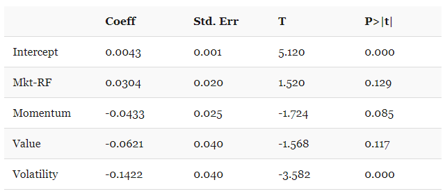
In the table below, we plot the results of regressing against the traditional Fama-French 3-Factor model.

We see that while the HML factor (i.e. value) is statistically significant (with a small negative loading), the intercept remains economically large and significant, indicating that seasonality remains unexplained.
We also wanted to explore whether the anomaly was subsumed by sector-specific implementations of different factor strategies. Specifically, we construct a value long/short, a momentum long/short, and a volatility long/short.
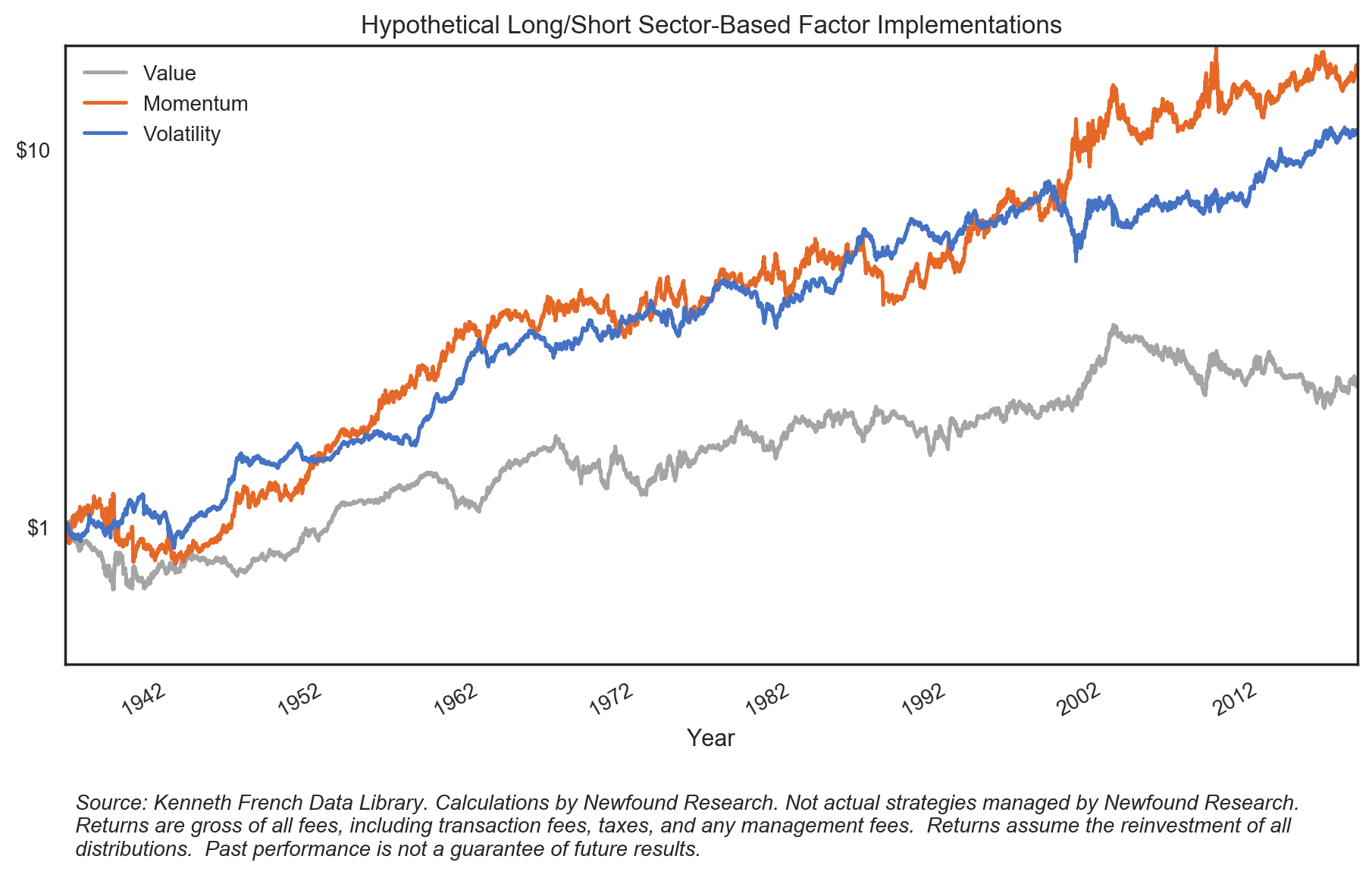
While the volatility anomaly appears significant, the intercept remains large and the anomaly remains unexplained.
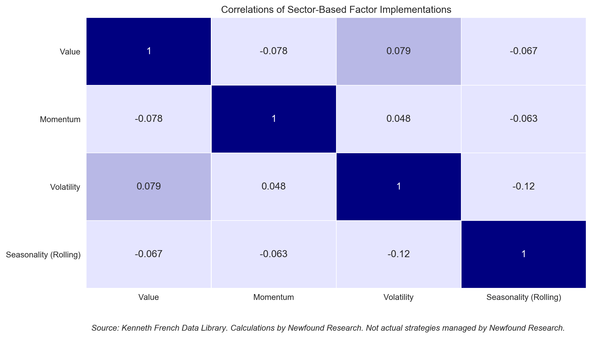
Evaluating correlations, we can see that for sector-based traders, seasonality may be a potentially valuable diversifier from traditional value, momentum, and volatility anomalies.
Finally, we wanted to explore whether the seasonality effect simply data-mined an advantageous average sector weighting over time? To answer this question, we regress the monthly returns of the long/short against the market’s excess returns as well as sector returns in excess of the market. This allows us to extract broad beta effects as well as industry specific effects.
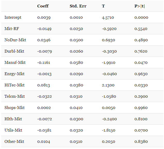
We see that the anomaly remains both large and significant, and only the Manufacturing and Technology sectors offer any explanatory significance, with a negative loading on the former and a positive loading on the latter. This indicates that at least part of the strategy’s edge may have come from being net short Manufacturing and net long Technology, on average.
Conclusion
We have demonstrated that seasonality in the U.S. sectors has been economically significant when measuring it using historical returns in previous months over the past 75 years. The effect is robust to the lookback window length and the lookback window type. It is also significant when accounting for other known anomalies (such as value, momentum, and size), sector-specific factors, and industry weights.
Despite this empirical evidence, we still do not know why seasonality is significant. Why should seasonality work in the future? What specifically has caused it to work in the past?
Without knowing the theoretical reason for an anomaly, be it behavioral, structural, or otherwise, it is difficult to rely on it going forward.
This is not to say that it won’t work – if it does, it may even diversify other investing styles. But until we can see more tests done with out-of-sample data, any seasonality strategy should likely garner only a small allocation within a well-diversified factor portfolio.
Corey Hoffstein is the Co-founder & CIO at Newfound Research, a participant in the ETF Strategist Channel.
- https://papers.ssrn.com/sol3/papers.cfm?abstract_id=3177539
- https://papers.ssrn.com/sol3/papers.cfm?abstract_id=2154873
- https://papers.ssrn.com/sol3/papers.cfm?abstract_id=2224246
- Long/short strategies go long the top 3 ranked sectors and short the bottom 3 ranked sectors. Value ranks are based upon 5-year z-scores of trailing twelve-month yields. Momentum ranks are based upon 12-1 month returns. Volatility ranks are based upon 63-day exponentially weighted realized volatility. Value and momentum are implemented in a dollar-neutral fashion, while volatility is implemented such that both long and short legs are of equal volatility. Each strategy is implemented using an overlapping portfolio approach, with value assuming 36 overlapping portfolios (rebalanced monthly), momentum assuming 4 overlapping portfolios (rebalanced weekly) and volatility assuming 26 overlapping portfolios (rebalanced weekly).