
Reducing fees by switching strategies is an uncertain savings. Maximizing the potential of the risk-free rate is guaranteed return.
Portfolio Construction and the Risk-Free Rate
One of the primary uses of the risk-free rate in portfolio construction is within a mean-variance framework where the goal is to maximize the expected Sharpe ratio. The effect of changing the risk-free rate is illustrated in the chart below.
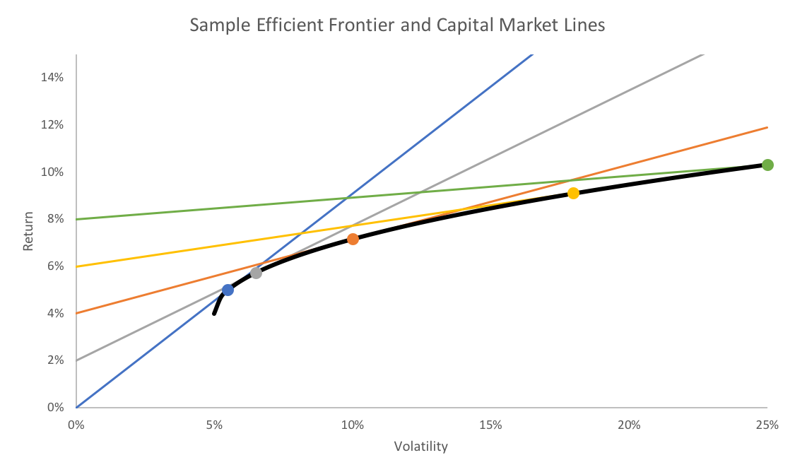
The efficient frontier is shown in black, the different capital market lines are shown as the colored lines, and the corresponding circles indicate the tangency portfolios.
All else held equal, a higher risk-free rate moves the tangency portfolios further out on the efficient frontier. From an implementation standpoint, an investor desiring to target a specified volatility level would hold some mix of the tangency portfolio and the risk-free asset.
A practical issue comes into play when we consider the assumptions behind modern portfolio theory: namely that borrowing and lending are done at the same rate.
Investors outside of larger institutional investors generally pay a premium for borrowing funds, and as we have seen from bank account data, receive potentially much less for lending.
As such, the borrowing line is likely to be more set in stone. For example, a larger account at Interactive Brokers would pay about 100 bps over the Federal Funds rate to borrow.
In the example above, if we assume that borrowing is done at 4% – the orange line – and lending (i.e. savings) is done at 0% – the blue line – then the capital market line actually is kinked along the efficient frontier.2
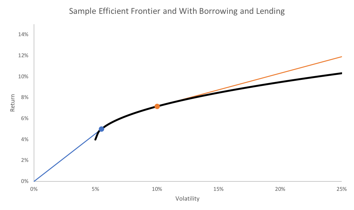
When you move up the blue line to the blue tangency portfolio, you then move along the efficient frontier because you cannot borrow at 0% and because of the risk-free rate being used, either by choice or not, you cannot lend at 4%. You move up the efficient frontier until you hit the orange tangency portfolio, at which point you begin to move along the orange line as you borrow at 4%.
Increasing your risk-free rate as much as possible shapes the capital market “line” as more of an actual line, which is desirable in the Sharpe-optimal framework.
The Practical Impact of the Risk-Free Rate
Using a cross-section of asset classes (including global equities, government bonds of various maturities, and commodities) going back to 1973, we can use different fractions of the risk-free rate and construct the implied long-only mean-variance optimal portfolios (using resampling to account for estimation noise). To obtain expected return and covariance estimates, we will use a 3-year forward crystal ball and form the portfolio each month. Even though we are using a crystal ball over a longer time horizon, the shorter holding period still may deviate considerably (a topic we discussed in a different context in God, Buffett, and the Three Oenophiles).

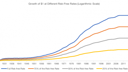
As of late, there has not been much difference in the rolling returns, which is expected given the extremely low risk-free rates. The largest benefit was in the 80s and 90s when rates were regularly above 5%.
Over the whole period, the annualized rates of return were 9.9%, 10.7%, and 11.8%, depending on whether a 0% risk-free rate, half of the risk-free rate, or the full risk-free rate was assumed.
Note that this analysis assumes that the investor will simply hold the mean-variance optimal portfolio with no regard to its volatility level. This means that the rolling returns may not compare apples-to-apples, as one portfolio may bear significantly more risk than another. In an effort to more accurately isolate the impact upon returns, we can attempt to hold volatility levels constant among the portfolios.
Since the borrowing rate for all portfolios is assumed to be the same, we will add cash in with the higher volatility portfolios to bring their forecast volatilities in line with the 0% risk-free rate portfolio. This avoids using leverage, which is in line with many investor processes. This results in a generally conservative portfolio (overall volatility of 7.5%).
A similar effect emerges, where the full risk-free rate portfolio gains ground when risk-free rates are high and loses ground when rates are lower.

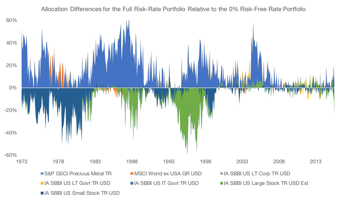
Over the 2000s, the portfolio with the full risk-free rate has been lagging the 0% risk-free rate portfolio, mainly because of the difference in the tangency portfolios’ performance for the two rate scenarios. The lower volatility portfolio has done well, and for much of the time, the tangency portfolios have been close to identical, as shown in the following chart.
Positive numbers indicate that the full risk-free rate portfolio had a higher allocation to that asset class, and vice versa.
Conclusion
The risk-free rate is commonly used and discussed in portfolio discussion without much definition or consideration beyond the fact that it exists.
There is no set risk-free rate, but there is a generally accepted ceiling that can be earned without taking any significant risk. There is however the unfortunate opportunity of earning 0% as your own personal risk-free rate.
In a mean-variance framework, the selected risk-free rate will have some bearing on the optimal portfolio and will affect the resulting mix of this portfolio and the risk-free asset. These effects have been most pronounced when the risk-free rate is higher.
With rates still low from a historical perspective, the impact of not achieving the full risk-free rate may not be extreme, but with how simple it is to deploy cash in a more effective manner, setting up a process in the current increasing rate environment is a sensible way to maximize returns in a guaranteed way when other assets are facing headwinds of uncertainty.
- Services like Max My Interest aim to make this bank account selection process simpler, especially for accounts above the FDIC coverage limit.
- See Lee M-C. and Su, L-E. Capital Market Line Based on Efficient Frontier of Portfolio with Borrowing and Lending Rate. Universal Journal of Accounting and Finance 2(4): 69-76, 2014. http://www.hrpub.org/download/20140801/UJAF1-12202421.pdf
Nathan Faber is Vice President at Newfound Research, a participant in the ETF Strategist Channel.