

By Canterbury Investment Management
Canterbury Portfolio Analytics
Tom Hardin, CMT, CFP, Chief Investment Officer
Brandon Bischof, Co-Director Canterbury Portfolio Analytics
Conventional wisdom dictates that financial markets behave in a random and normally distributed pattern. Conventional wisdom also holds that portfolio management decisions be determined based on the investor’s risk tolerance and personal financial objectives.
The Canterbury Portfolio Thermostat relies on a different set of assumptions. Markets are not random and normally distributed and portfolio decisions should not be based on subjective view of investor’s risk tolerance and personal objectives, but instead decisions should be made based on creating the most efficient portfolio that matches the existing market environment. The Portfolio’s allocation, diversification, security selection, and construction should adapt to move in concert with the dynamic market environments- bull or bear.
This paper will take a hard look at some keystone assumptions that are the basis behind traditional portfolio management practices. Canterbury studies provide statistically relevant evidence that markets are not random, but instead experience many different market environments, called Market States.
What is a Market State?
Identifying the macro stock market environment is the first step in the Canterbury Portfolio Thermostat Process. The Portfolio Thermostat process combines volatility and a combination of supply and demand indicators to identify the current state of market efficiency. Using daily data, the system has been tested back to 1896 (32,000 data points) and confirmed 12 different Market State environments. They are categorized as:
- 5 Bullish (rational) Market States
- 4 Bearish (irrational) Market States
- 3 Transitional Market States (which tend to precede a change from Bullish to Bearish, or vice versa, indicating caution)
3 Primary Inputs to Market States:
- Long-Term Indicators: Identify the long-term status of the market or security.
- The Canterbury Volatility Index (CVI): Evaluate the degree of rationality/efficiency of the current market environment. An “efficient market” environment is one that is marked by low or declining volatility. Efficient markets should have limited risk similar to a normal bull market correction, defined as a 10% decline from the peak value.
- Short-Term Supply & Demand Indicators: Indicate the short-term directional movement of the current market.
The following Chart (Figure 1) shows the characteristics of each of the 12 Market States.
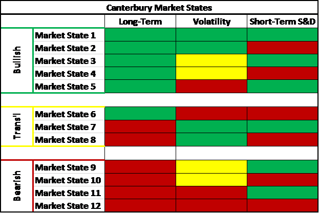
Figure 1: Canterbury Market States
What Does Each Market State Environment Mean?
Market State environments are not about the predictability of return, but rather the level the of risk that can be expected. Each Market State environment exhibits its own unique characteristics, associated with a given risk. Risk is defined as Volatility and Drawdown (the maximum decline from peak to trough).
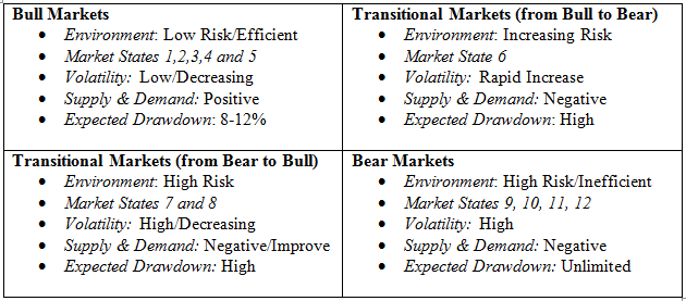
Table 1: Environment Characteristics
The table above (Table 1) shows characteristics of each of Market State environment. Notice the expected drawdown for each environment. In Bullish Market State environments, risk is typically limited to about 8-12%. In transitional environments, risk is high, but can either be increasing or decreasing as the market shifts to either Bullish or Bearish. Bearish Market State environments have unlimited risk for loss. We can see this displayed in Figure 2.
Figure 2 shows the daily prices of the S&P 500 from 1950 to April 10, 2018 with Market State environments.
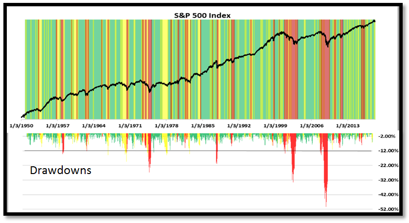
Figure 2: S&P 500 with Market Environments & Drawdowns
The colored background in Figure 2 highlights the Market State environment each day. Bullish Market State environments are green; Transitional Market State environments are yellow; Bearish Market State environments are red. The bottom half of the Figure 2 displays the drawdowns (percentage decline from the peak) within each Market State environment period. Notice that most of the Bull Market State declines are less than the expected -12%, as opposed to Transitional and Bearish Market State environments, which can exceed -20%, -30%, and beyond.
During Canterbury’s identified bull markets, there are considerable gains made on the market. While Market State environments do not identify return directly, Bull markets, which are periods of low risk, are often periods of high returns with limited downside.
Market State Environment Statistics
Canterbury has daily data, on the S&P 500, that goes back to 1950. Canterbury ‘s Portfolio Analytics Group has identified the daily Market State and Canterbury Volatility Index (CVI) volatility for every day (17,000 days). Table 2 shows some interesting statistics for each Market State environment (Transitional Markets and Bear Markets are combined due to their high-risk trait). Keep in mind that Bull markets are categorized by low volatility and low risk; Bear markets have high volatility and unlimited risk.
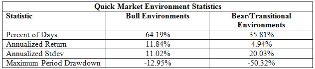
Table 2: Quick Market State Environment Stats
Table 2 shows that Market State environments are characterized by low volatility and stability. These same characteristics are held true for markets and Individual securities. Transitional and Bear Market State environments had many substantial declines. Bull Market State environments had higher returns verses risk taken (as measured by standard deviation). Thus, Bull markets have smaller drawdown (dollar declines), allowing for more efficient long-term compounding of returns.
The most efficient portfolio is the one that has the highest return verses risk taken. Since markets are dynamic and will experience both bull and bear markets, there is no single fixed percentage asset allocation model that will consistently produce an efficient portfolio that can withstand dynamic markets. The most efficient portfolio is a moving target. In other words, the combination of securities that produced a low risk/high return portfolio in 2017 (a Bullish Market State environment) would have been very inefficient during 2008 (a Bearish Market State environment).
Markets & the Bell Curve
Academia and most Nobel Laurites in Economics say the stock market may be thought of as being “random” and having “normal distribution.” However, Canterbury has conclusive evidence debunking both pieces of conventional wisdom. In fact, the same studies confirm that it is possible to identify the difference between low-risk Bull and high-risk Bear markets.
Canterbury tested the daily data, on the S&P 500, from the beginning of 1950 to April 10th, 2018 (16,977 days). The daily standard deviation was calculated to be 0.96%. This would mean a normal distribution of random daily returns would occur in the market as follows (Table 3):
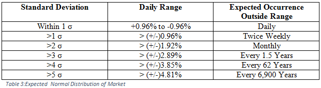
The actual results revealed little to no statistical evidence that markets are random or normally distributed. As the number of standard deviations increases, the bell curves probabilities of expected results become further removed from the reality of what actual markets produce.
The following is a summary of the increasing gap between the bell curves expected results and the reality of how markets behave (Table 4):
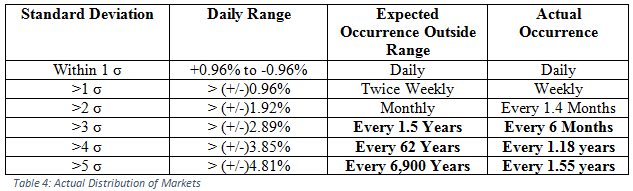
Table 3 and Table 4 show that 3rd standard deviation events, and higher, occur much more frequently than what a normal distribution bell curve would predict. For example, a third standard deviation day (a day beyond +/- 2.89%) should only happen every 1.5 years, but in reality, 3rd standard deviation days happen twice per year on average. 5th standard deviation days should only occur once every 6,900 years, yet in reality they occur much more frequently: 1 in every 1.5 years. Markets have too many outliers that occur to fit the normal bell curve.
Summary of Markets and the Bell Curve:
Canterbury studies that there is no statistical relevance between the bell curve generated probabilities and the more erratic behavior of markets. The difference between the projected probability of results and the actual results are so far apart that they have no statistical relevance.
Markets States and the Bell Curve:
In addition, Canterbury studies provide conclusive results that show that market outliers are in fact not random, but more likely to occur when certain market characteristics are in place. In other words, outliers occur much more frequently during Canterbury’s 4 Bear Market States and much less frequently in the 5 Bull Market States.
Table 5 shows the distribution in Bull Markets (10,898 days) assuming the market’s overall daily standard deviation of 0.96%.
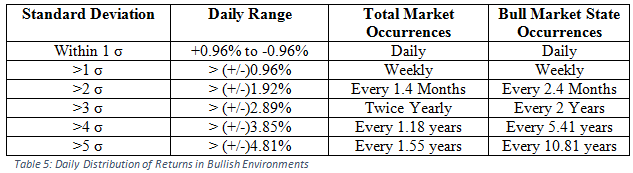
The 5 Bullish Market State environments have a significantly high number of days that fall within the first standard deviation (85%) than what the bell curve would predict (68%). On the other hand, the number of outliers, beyond a 3rd standard deviation, which occur frequently in the market, are much less likely and tend to be smaller in Bull Market States.
Conversely, the 4 Bear Market States have many more daily outliers beyond a 3rd standard deviation than what occur during the 5 Bull Market States.
Table 6 shows Bear Market distributions (2,181 days).

Bear markets are known for extreme high volatility. One day events, beyond a 3rd standard deviation that should occur every 1.5 years, actually occur on a monthly basis during Bear Market States. Meanwhile, 4th and 5th standard deviation events, which should be incredibly unlikely, can be expected on a quarterly basis during Canterbury Bear Market States. One observation Canterbury has made on Bear Market State environments is that both the largest down days and largest up days happen in Bear Market States.
Bear markets display a vast number of erratic movements that are more random and risky than that of a Bull Market States.
Conclusion
The bell curve is best for measuring the probabilities of a result within a closed system, for example, flipping a coin or a rolling a die, (the result will be between 1 to 6). Markets, on the other hand, are an open system, meaning that there are no meaningful restraints on the size or frequency of the daily fluctuations. As a result, more and larger outlier days should occur more frequently than what bell curve probabilities would predict.
Given that markets are not random nor normally distributed, then the daily fluctuations would be a direct result of the interaction between cause and effect. Markets are driven by the law of supply and demand. The changing forces of supply and demand are driven by investor actions, which in turn are based their predictions regarding the future and how convicted they are that they will be correct. Investor beliefs and emotions will change over time. Increased volatility and outliers are the result of the emotional actions of likeminded investors.
According to Canterbury studies, the majority of outlier days are preceded by an increase in volatility. Outliers become more frequent as volatility continues to increase. Therefore, a leading indicator of future market outliers is an increase in volatility.
Volatility, Outliers, and Drawdowns
The following is a Market State study on volatility and outlier days:
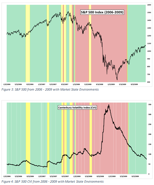
Figure 3 depicts the S&P 500 from 2006-2009 as well as its Market State environments. This period was chosen to look at because it goes from Bullish to Transitional to Bearish and back to Bullish. Figure 4 shows the Canterbury Volatility Index(CVI) over the same time frame. Notice how CVI and the Market are inversely correlated. Figure 5 shows S&P 500 drawdowns during the period while in each market state. Notice that when the S&P 500 Index is in one of the Bull Market State environments, CVI is generally low and the drawdowns are typically limited to normal market noise of 10% or less. Conversely, during Transitional and Bear Market State environments, CVI is mostly high or increasing and drawdowns are larger.
This article was submitted by Canterbury Investment Management, a participant in the ETF Strategist Channel.