

By Mark Kritzman and Cel Kulasekaran
Whether the continuing trend to ESG oriented investment is motivated by a desire to do good or the expectation of flow-driven superior performance, exposure to risky assets still carries the risk of significant drawdowns, even for assets that deliver superior relative performance. It may therefore be prudent to approach ESG investing within a risk management framework that cuts risk when market conditions are fragile and adds risk when market conditions are resilient. The challenge, of course, is to know when conditions are fragile and when they are resilient.
Traditional risk indicators such as implied volatility, credit spreads, and term spreads have a mixed record of distinguishing fragile markets from resilient markets. There are, however, two risk indicators that have emerged from the academic literature and have been embraced by the investment community and policymakers that may, on average, offer a reasonably reliable forewarning of shifting risk conditions. The first indicator is a measure of risk concentration called the Absorption Ratio, and the second is a measure of the statistical similarity of prevailing conditions to past episodes of market weakness, based on a statistic called the Mahalanobis distance.
Risk Concentration
The Absorption Ratio gives the fraction of variability across equity sector returns explained by a group of key factors which are identified by principal components analysis. A high Absorption Ratio indicates markets are tightly coupled, in which case they are fragile because negative shocks travel more quickly and broadly than when markets are loosely linked. A low Absorption Ratio indicates that risk is broadly distributed across many separate sources. When markets are in this state, they are more resilient to shocks and less likely to exhibit a systemic response to bad news.
Consider, for example, a sudden rise in energy process when risk is diffused. We might expect the price of airline stocks to decline because their operating expenses have risen unexpectedly. But we would not expect this jump in energy prices to travel to other parts of the market that are not fundamentally linked to energy prices. However, if market conditions are tightly coupled, it would not be unusual to observe a market wide decline in prices following an unanticipated spike in energy prices.
One might assume that the average correlation of stocks would yield similar information. However, the Absorption Ratio is a more informative measure of risk concentration than average correlation because average correlation fails to account for the relative importance of assets. A change in the correlation of two assets with relatively low volatility is less relevant to risk concentration than a change in the correlation of two relatively high-volatility assets. The Absorption Ratio, by construction, precisely accounts for the relative volatility of the assets.
Exhibit 1 shows the left 10th percentile tail of weekly U.S. equity returns. The curved line shows the full sample left tail assuming a normal distribution based on the empirical mean and standard deviation. The blue bars represent the empirical left tail following a standardized shift in the Absorption Ratio of less than of -1, indicating resilient market conditions. The orange bars represent the empirical left tail following a standardized shift in the Absorption Ratio of greater than +1, indicating fragile market conditions. Exhibit 1 starkly reveals that the frequency of losses was much lower following a shift down in the Absorption Ratio compared to the expectation of losses from the full sample mean and standard deviation, while the frequency of losses following a spike up in the Absorption Ratio was much higher than the full sample mean and standard deviation would imply.
Exhibit 1: 10th Percentile Left Tail of Weekly U.S. Equity Returns
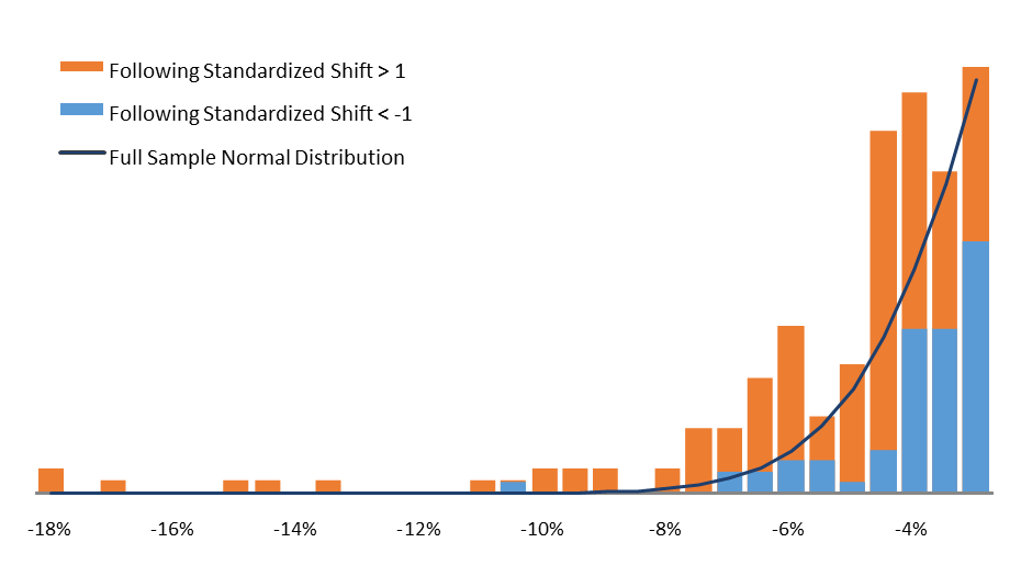
Source: Kinlaw, W., M. Kritzman, and D. Turkington. “Toward Determining Systemic Importance” The Journal of Portfolio Management. Summer 2012.
Both policymakers and industry researchers have offered supportive views of the efficacy of the Absorption Ratio. For example, the U.S. Treasury Department concluded that the Absorption Ratio would have given advance warning of financial crises as far back as the 1920s.
“For the 1998 crisis, in which tight coupling of other markets to the Russian bond market caught LTCM by surprise, there was a gradual increase in the AR before the event and a gradual decrease after. Similarly, the AR rose gradually up to September 2008 but then jumped abruptly by more than 10 percent and remained elevated for two years. There was a similar pattern in 1929.”
Source: Office of Financial Research Annual Report 2012. United States Treasury Department. Page 43.
The Absorption Ratio has also gained traction in the investment industry. A report by Citigroup stated that the efficacy of the Absorption Ratio extends to European markets as well as equity sectors.
“Our findings suggest that the Absorption Ratio certainly has some merit as a market timing signal in Europe and we see it as a useful tool for identifying market fragility/systemic risk. Additionally, we extend the application of the Absorption Ratio to sector timing/rotation. Using the methodology within sector at the stock level, we find that Absorption Ratio could be used successfully in timing sector rotation.”
Source: Citi Investment Research & Analysis – Under the Microscope Report 2010. Citigroup Global Markets. Page 1.
Exhibit 2 shows the annualized spread of U.S. stock performance when conditioned on the Absorption Ratio[1]. It shows an inverse relationship between stocks and U.S. Treasuries. These spreads persist over the subsequent 5-day and 10-day periods for both asset classes.
Exhibit 2: Risk Concentration Conditional Returns
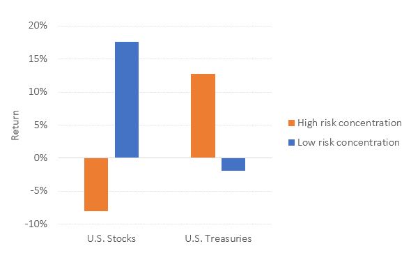
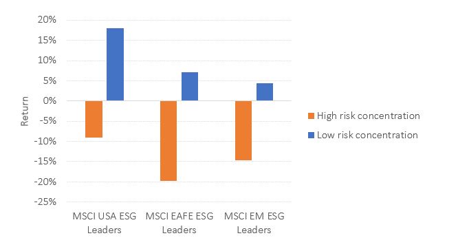
Exhibit 3 shows the application of the Absorption Ratio and the corresponding behavior of ESG stocks when conditioned on the Absorption Ratio. It reveals a similar inverse relationship.
Exhibit 3: Conditional Performance of ESG Stocks (using Risk Concentration)
Risk Similarity
As mentioned previously, we can use a statistic called the Mahalanobis distance to measure the statistical similarity of current global asset class conditions to past periods in which global equities suffered significant losses. The Mahalanobis distance was originally derived to analyze human skulls, but it has since been applied in a wide variety of fields including finance, engineering, and medicine, to name but a few. Unlike the standard Euclidean distance, the Mahalanobis distance accounts for the variances and correlations of variables. All else equal, two observations are more distant if the spread between their values is large compared to the typical variation of those values. And all else equal, two observations are more distant if the pattern of differences between their values diverges from the typical pattern of differences in values. The Mahalanobis distance neatly summarizes all the information from a covariance matrix in a single number.
Exhibit 4 reveals that U.S. stocks had much lower annualized returns during periods that were statistically similar to periods of market weakness[2] as measured across global asset classes than during periods that were not similar to periods of market weakness. And it reveals the opposite relationship for U.S. Treasuries, which we should expect from a safe alternative to equities.
Exhibit 4: Risk Similarity Conditional Returns[3]
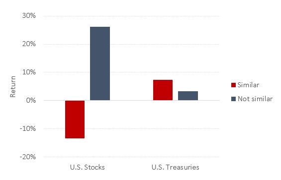
Exhibit 5 shows that this pattern carries over to ESG equities in the developed U.S. market, the developed non-U.S. markets, and the emerging markets. ESG equity performance was much worse during periods that were statistically similar to periods of market weakness than during periods that were not similar to periods market weakness.
Exhibit 5: Conditional Performance of ESG Stocks

Conclusion
Whether ESG equity investors are motivated by the desire to do good or the expectation of superior performance, they face the prospect of potential selloffs merely by virtue of their exposure to risk. We therefore propose that ESG equity investors consider adding a dynamic component to their portfolios that cuts risk when market conditions are fragile and accepts risk when conditions are resilient.
Additionally, we propose that ESG equity investors consider two risk indicators to distinguish fragile markets from resilient markets: the Absorption Ratio which measures risk concentration, and risk similarity which measures the statistical similarity of prevailing conditions to past periods of market weakness. We offered persuasive evidence of the efficacy of these risk indicators.
[1] We use the Wilshire 5000 Total Return Index for U.S. stocks and the Bloomberg U.S. Treasury Total Return Index for U.S. Treasuries. We calculate the contemporaneous returns conditioned on a high risk concentration from October 2007 through May 2022. We use October 2007 as a start date to coincide with common dates of ESG index data across exhibits. We consider high risk concentration as the 90th percentile rank or greater of the absorption ratio, over a moving 1-year window; conversely we consider low risk concentration as the 10th percentile rank or lower of the absorption ratio.
[2] Windham measures risk similarity by calculating the statistical similarity of global asset class returns across equities, fixed income, real estate, and commodities to periods of weak global equity performance (one standard deviation below its mean).
[3] We use the Wilshire 5000 Total Return Index for U.S. stocks and the Bloomberg U.S. Treasury Total Return Index for U.S. Treasuries and calculate the contemporaneous returns conditioned on statistical risk similarity to weak global equity weak markets from October 2007 through May 2022. We use October 2007 as a start date to coincide with common dates of ESG index data across exhibits.